Tuning Random Forest with Grid Search

In machine learning, models require fine-tuning of their hyperparameters to reach their full potential. This process, known as hyperparameter tuning, is essential for enhancing a model’s performance, including for algorithms like Random Forest.

Random Forest, a versatile and robust algorithm, excels in both classification and regression tasks, making it a favorite among data scientists. However, finding the right combination of hyperparameters for a Random Forest can be challenging. That’s where Grid Search, a systematic approach to hyperparameter tuning and optimization, comes in.

In this article, we’ll discuss how to find the best set of hyperparameters for Random Forests using Grid Search. Along the way, we’ll show practical examples in Python using sklearn.

Master hyperparameter optimization with grid search (and other methods), with our course Hyperparameter Optimization for Machine Learning.

Let’s start by discussing what hyperparameter tuning is, and the methods commonly used to optimize machine learning models.

Hyperparameter tuning methods

Hyperparameter tuning is commonly used in machine learning to improve a model’s performance. By adjusting model hyperparameters like n_estimators or max_depth for tree-based models, learning rate or number of epochs for neural networks, or number of clusters in the k-means algorithm, we can optimize how the algorithm learns and generalizes to new data.

Proper tuning helps achieve the best results on both the training set and also test data, hence preventing overfitting or underfitting.

Depending on the problem’s complexity and the number of hyperparameters involved, we can apply different tuning techniques to efficiently find the optimal set of hyperparameters. Each method tries to find the set of hyperparameters that maximizes a model’s performance.

Some common methods for hyperparameter tuning are:

• Manual Search: During manual search, we adjust hyperparameters by trial and error, manually. This method is intuitive but inefficient and time-consuming.
• Grid Search: During grid search, we test all combinations of hyperparameters using cross-validation to identify the set of hyperparameters that result in the best model performance.
• Randomized Search: In a randomized search, we evaluate random hyperparameter combinations, which are sampled from distributions of hyperparameter values, offering faster results while still covering a broad parameter space.
• Bayesian Optimization: This method tries to predict the best hyperparameters using probability models, making it efficient for larger and more complex algorithms, that take longer to train.

Watch detailed tutorials about the various hyperparameter tuning techniques, in our course Hyperparameter Optimization for Machine Learning.

Grid Search is a widely used hyperparameter optimization method due to its simplicity and comprehensive exploration of the hyperparameter grid. It is particularly useful for relatively simple models like Random Forest.

Grid Search

Grid Search is a popular method for hyperparameter tuning in machine learning. It automates the process of searching for the best combination of hyperparameters to optimize a machine learning model. Instead of manually adjusting each hyperparameter, Grid Search explores all possible combinations in a given parameter grid and identifies the one that results in the best performance.

In simple terms, imagine you have multiple hyperparameters with different possible values; Grid Search evaluates every possible combination of these values, helping you find the optimal set of hyperparameters for your model.

How Does the Grid Search Algorithm Work?

Grid Search tests every possible combination of hyperparameters within a parameter grid. A parameter grid is simply a dictionary where the keys are hyperparameter names and the values are lists of possible values for each hyperparameter. For instance, while tuning a Decision Tree classifier, the parameter grid might look like this:

param_grid = {
    'max_depth': [3, 5, 10, None],
    'min_samples_split': [2, 5, 10],
    'criterion': ['gini', 'entropy']
}

The Grid Search algorithm evaluates all possible combinations of the hyperparameters within the grid. For the above-specified grid, the algorithm will evaluate 4x3x2 combinations:

• Max_depth : 4 options (5,3,10,None)
• min_sample_split: 3 options (2,5,10)
• criterion: 2 options (‘gini, ‘entropy’)

Total combinations : 4 x 3 x 2 = 24

This means that the Grid Search algorithm will train and test the model 24 times, selecting one value from each hyperparameter and repeating the process until all values of that hyperparameter are combined with all the values of the rest of the hyperparameters.

For instance, max_depth=3 will be combined in the following way with the other hyperparameters:

• max_depth = 3, min_samples_split = 2, criterion = ‘gini’
• max_depth = 3, min_samples_split = 2, criterion = ‘entropy’
• max_depth = 3, min_samples_split = 5, criterion = ‘gini’
• max_depth = 3, min_samples_split = 5, criterion = ‘entropy’
• max_depth = 3, min_samples_split = 10, criterion = ‘gini’
• max_depth = 3, min_samples_split = 10, criterion = ‘entropy’

The same combinations are repeated for the other values of max_depth (i.e. 5, 10 and None). Using cross-validation, all these combinations are trained and tested on different subsets of the training data.

Master Grid Search with our tutorials at Hyperparameter Optimization for Machine Learning.

Cross-validation

Cross-validationis a popular technique for validating a model’s performance. It splits the training data into several smaller subsets, called folds. The model is trained on some of these folds and tested on the remaining one, ensuring that each data subset is used for training and testing. This process helps prevent overfitting and ensures that the model performs well on unseen data, providing a more accurate estimate of its performance.

Grid Search uses K-fold cross-validation, where the data is divided into K folds. The model is trained on K-1 folds and evaluated on the remaining fold through multiple iterations. Grid Search calculates the average performance across all folds to provide a final score for each combination of hyperparameters. This score is based on an evaluation metric that determines the model’s performance. By default, Grid Search uses the model’s scoring method, which varies depending on the type of model and task (classification or regression). However, a custom scoring metric can also be specified while using the algorithm.

So, for our parameter grid with 3 hyperparamater combinations (max_depth, min_sample_split, criterion), if 5-fold cross-validation is used, then the model will be trained and validated 24×5 = 120 times or (4x3x2) x 5 = 120 times.

Now, let’s understand how the Grid Search algorithm works with the help of an example. Consider the following set of hyperparameters of a Decision tree classifier:

max_depth = 3 min_sample_split = 5 criterion = ‘gini’

Assuming that we are using 5-fold cross-validation (K=5) and our training data has 100 samples, the algorithm works like this:

1. Split the Data into K Folds: Split the 100 samples into 5 folds (i.e., 5 subsets of the data). Each fold will contain 20 samples. So, the dataset looks like this:
   • Fold 1: Samples 1 to 20
   • Fold 2: Samples 21 to 40
   • Fold 3: Samples 41 to 60
   • Fold 4: Samples 61 to 80
   • Fold 5: Samples 81 to 100
2. Train and Test on Different Folds: For the combination (max_depth=3, min_samples_split=5, criterion=’gini’), GridSearchCV will use the first fold (Samples 1 to 20) for testing and the remaining 4 folds (Samples 21 to 100) for training. It will fit the Decision Tree model on the training data (Samples 21 to 100) and test it on Fold 1 (Samples 1 to 20). It will then calculate the accuracy score (default metric for classification) for this combination of hyperparameters.
3. Repeat the Process for All Folds: Now, GridSearchCV will rotate the folds so that each fold gets a chance to be the test set while the other folds are used for training. For instance,
   • Second iteration: Test on Fold 2 (Samples 21 to 40), train on the remaining data (Samples 1-20, 41-100)
   • Third iteration: Test on Fold 3 (Samples 41 to 60), train on the remaining data (Samples 1-40, 61-100).
   • and so on…

4. Calculate Average Performance: After testing on all 5 folds, GridSearchCV averages the evaluation metric (e.g., accuracy) from each fold. This gives a final performance score for the combination (3, 5, ‘gini’) across all folds. For instance, let’s say the accuracy scores of the 5 folds are [0.85, 0.87, 0.83, 0.88, 0.86], then the mean cross-validation score for that combination of hyperparameters will be 0.858.

5. Best Score: GridSearchCV repeats all the above steps for all possible hyperparameter combinations from the parameter grid. Once all combinations are tested, GridSearchCV identifies the highest mean score across all folds and all hyperparameter combinations, finally resulting in a set of hyperparameters that gives the best model performance.

Now that we know what is Grid Search and how it works, let’s jump onto understanding the hyperparameters of Random Forest and how we can utilize Grid Search to tune a Random Forest model.

Tuning Random Forest with Grid Search

Random Forest is a widely used ensemble learning method in machine learning that performs exceptionally well in both classification and regression tasks. It builds multiple decision trees during training and combines their individual predictions to create a more accurate and stable model. By averaging the outcomes (for regression) or taking a majority vote (for classification), Random Forest helps reduce overfitting and increases model accuracy.

Random forest is made up of multiple decision trees where each tree is trained on a random subset of data (using bootstrapping). At each split, the algorithm considers a random subset of features to introduce variability among trees. Finally, it combines the predictions from individual trees to make the final prediction, increasing accuracy and reducing variance.

While Random Forest is a powerful algorithm, its performance can vary significantly based on the choice of hyperparameters. For example, the number of trees (n_estimators) and the maximum depth of each tree (max_depth) directly influence the model’s accuracy and generalization ability. Without selecting the right hyperparameters, the model may either overfit or underfit the data. Too many trees or very deep trees can lead to overfitting, while too few trees or shallow trees may cause underfitting.

Some of the key hyperparameters that significantly affect the performance of a Random Forest model include:

• n_estimators: The number of trees in the forest. More trees typically improve model accuracy but increase computational cost.
• max_depth: The maximum depth of each decision tree. Limiting depth helps prevent overfitting.
• max_features: The number of features to consider for the best split at each node. It controls the diversity of the trees.
• min_samples_split: The minimum number of samples required to split an internal node. Higher values prevent the model from learning overly specific patterns.

• min_samples_leaf: The minimum number of samples required to be at a leaf node. Setting this value higher can smooth the model and reduce overfitting.

• criterion: The function used to measure the quality of a split, such as “gini” for classification or “mse” for regression.
• random_state: Controls the randomness of the training process, ensuring reproducibility.

For a detailed overview of the above hyperparameters in Random Forest, you can check out the “Ensemble Algorithms” section in our blog on Hyperparameters in Machine learning.

By understanding these hyperparameters, we can see how each one influences the performance of a Random Forest model. To demonstrate this, let’s train a Random Forest model using default values of hyperparameters. This will serve as a baseline, which we’ll later compare with the performance of the GridSearchCV-tuned model.

We’ll use a Github’s alternative to the Heart Disease UCI dataset from Kaggle for the sake of importing the data directly via URL. The data is licensed and free to use.

Let’s load the necessary libraries and prepare the data for our model:

import pandas as pd

# Load the dataset directly from a URL
url = "https://raw.githubusercontent.com/Ankit152/Heart-Disease-Prediction/master/heart.csv"
data = pd.read_csv(url)

# Define features and target
X = data.drop('target', axis=1)
y = data['target']

# Split the data into training and test sets
X_train, X_test, y_train, y_test = train_test_split(X, y, test_size=0.2, random_state=42)

data.head()

The output of the above code is:

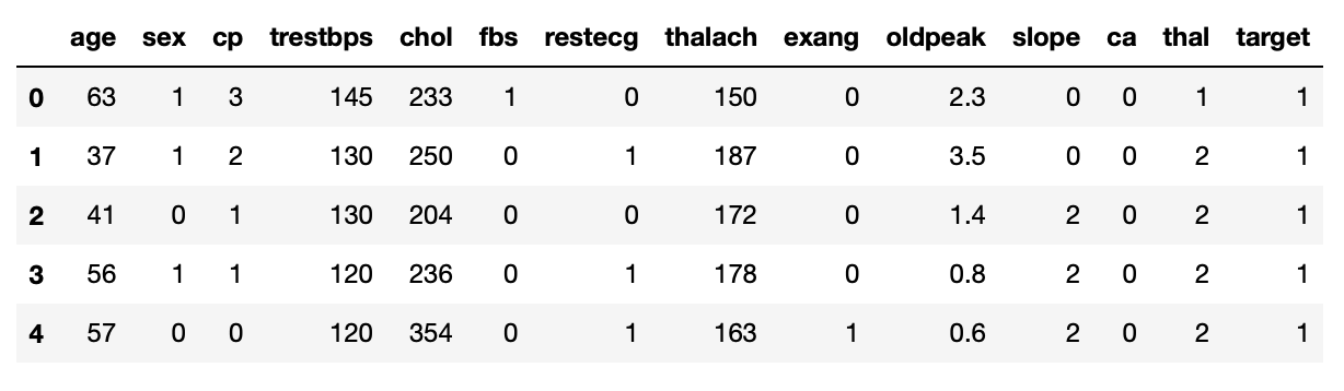
Now, that we have loaded the dataset, let’s jump into training the Random Forest Classifier by manually tuning the hyperparameters. We will evaluate the Accuracy and ROC-AUC along with mean and standard error with Cross-validation and a test set. These would be our baseline model metrics, which we will compare with the Grid Search model.

from sklearn.model_selection import cross_val_score
from sklearn.metrics import roc_auc_score, make_scorer
import numpy as np

# Initialize the Random Forest model with default hyperparameters
rf_model = RandomForestClassifier(
    n_estimators=100,
    max_depth=None,
    min_samples_split=2,
    min_samples_leaf=1,
    max_features='sqrt',
    random_state=42
)

# Cross-validation for accuracy
accuracy_scores = cross_val_score(rf_model, X_train, y_train, cv=5, scoring='accuracy')
mean_accuracy = np.mean(accuracy_scores)
std_accuracy = np.std(accuracy_scores)

# Cross-validation for ROC-AUC
roc_auc_scores = cross_val_score(rf_model, X_train, y_train, cv=5, scoring=make_scorer(roc_auc_score))
mean_roc_auc = np.mean(roc_auc_scores)
std_roc_auc = np.std(roc_auc_scores)

# Train the model on the full training data
rf_model.fit(X_train, y_train)

# Make predictions
y_pred_manual = rf_model.predict(X_test)
y_pred_prob_manual = rf_model.predict_proba(X_test)[:, 1]  # For ROC-AUC

# Calculate accuracy and ROC-AUC on the test set
accuracy_test = accuracy_score(y_test, y_pred_manual)
roc_auc_test = roc_auc_score(y_test, y_pred_prob_manual)

# Display results
print(f"Cross-validation Accuracy: {mean_accuracy:.4f} ± {std_accuracy:.4f}")
print(f"Cross-validation ROC-AUC: {mean_roc_auc:.4f} ± {std_roc_auc:.4f}")
print(f"Test Accuracy: {accuracy_test:.4f}")
print(f"Test ROC-AUC: {roc_auc_test:.4f}")

The output of the above code is:

Cross-validation Accuracy: 0.8058 ± 0.0100
Cross-validation ROC-AUC: 0.8022 ± 0.0065
Test Accuracy: 0.8361
Test ROC-AUC: 0.9186

The baseline model shows a cross-validation accuracy of 80.58%, with a small standard error of 1.00%, indicating stable performance across folds. The cross-validation ROC-AUC is 0.8022 with a standard error of 0.0065, reflecting the model’s capability to distinguish between classes. On the test set, the model achieves test accuracy of 83.61% and a test ROC-AUC of 0.9186, demonstrating good generalization ability

Now it’s time to evaluate how tuning impacts the model’s performance. Using sklearn GridSearchCV with cross-validation, we’ll systematically explore a predefined range of hyperparameters and find the optimal combination of hyperparameters for our model.

Below is the Python code to build and evaluate a Random Forest Classifier with GridSearchCV:

from sklearn.ensemble import RandomForestClassifier
from sklearn.model_selection import train_test_split, GridSearchCV
from sklearn.metrics import accuracy_score, roc_auc_score, make_scorer
import numpy as np

# Define the parameter grid for GridSearchCV
param_grid = {
    'n_estimators': [50, 100, 150],
    'max_depth': [None, 10, 20],
    'min_samples_split': [2, 5, 10],
    'min_samples_leaf': [1, 2, 4],
    'max_features': ['sqrt', 'log2', None]
}

# Initialize the Random Forest model
rf_model = RandomForestClassifier(random_state=42)

# Set up GridSearchCV
grid_search = GridSearchCV(estimator=rf_model,
                           param_grid=param_grid,
                           cv=5,
                           n_jobs=-1,
                           scoring='accuracy')

# Fit GridSearchCV to the training data
grid_search.fit(X_train, y_train)

# Get the best model from GridSearchCV and make predictions
best_rf_model = grid_search.best_estimator_
y_pred_gs = best_rf_model.predict(X_test)
y_pred_prob_gs = best_rf_model.predict_proba(X_test)[:, 1]  # For ROC-AUC

# Calculate accuracy and ROC-AUC for the best model
accuracy = accuracy_score(y_test, y_pred_gs)
roc_auc = roc_auc_score(y_test, y_pred_prob_gs)

# Cross-validation for accuracy and ROC-AUC
accuracy_scores = grid_search.cv_results_['mean_test_score']
mean_accuracy = np.mean(accuracy_scores)
std_accuracy = np.std(accuracy_scores)

roc_auc_scores = cross_val_score(best_rf_model, X_train, y_train, cv=5, scoring=make_scorer(roc_auc_score))
mean_roc_auc = np.mean(roc_auc_scores)
std_roc_auc = np.std(roc_auc_scores)

# Display results
print(f"Best Hyperparameters from Grid Search: {grid_search.best_params_}")
print(f"Cross-validation Accuracy: {mean_accuracy:.4f} ± {std_accuracy:.4f}")
print(f"Cross-validation ROC-AUC: {mean_roc_auc:.4f} ± {std_roc_auc:.4f}")
print(f"Test Accuracy: {accuracy:.4f}")
print(f"Test ROC-AUC: {roc_auc:.4f}")

The output of the above code is:

Best Hyperparameters from Grid Search: {'max_depth': None, 'max_features': 'sqrt', 'min_samples_leaf': 4, 'min_samples_split': 10, 'n_estimators': 50}
Cross-validation Accuracy: 0.8018 ± 0.0065
Cross-validation ROC-AUC: 0.8044 ± 0.0221
Test Accuracy: 0.8525
Test ROC-AUC: 0.9256

The Grid Search-tuned model demonstrates a cross-validation accuracy of 80.18%, with a small standard error of 0.65%. The cross-validation ROC-AUC is slightly higher than the baseline at 0.8044, but with a higher standard error of 0.0221, indicating a bit more variability across folds. The test accuracy improves to 85.25%, and the test ROC-AUCincreases to 0.9256, showing significant improvement in classification performance after hyperparameter tuning.

The baseline model shows good test accuracy (83.61%) and test ROC-AUC (0.9186), suggesting that it performs well out of the box. However, after applying Grid Search to optimize hyperparameters, the test accuracy increases to 85.25%, and the test ROC-AUC rises to 0.9256, indicating a better ability to distinguish between classes and handle class imbalances more effectively. The tuning process leads to a reduction in the standard error for cross-validation accuracy, from 1.00% in the baseline model to 0.65% in the Grid Search model, which highlights the increased stability and consistency of the tuned model’s performance across different folds.

To better understand the effect of hyperparameters on model performance, we visualize how changes in key parameters, such as the number of estimators, maximum depth, and minimum samples split among others, impact the model’s accuracy score:

import matplotlib.pyplot as plt
import seaborn as sns
import pandas as pd

# Assuming grid_search.cv_results_ contains the results of GridSearchCV
results = pd.DataFrame(grid_search.cv_results_)

# Set up the figure with 2 rows and 2 columns
plt.figure(figsize=(14, 10))

# Plot 1: Performance vs n_estimators
plt.subplot(2, 2, 1)
sns.lineplot(data=results, x='param_n_estimators', y='mean_test_score', marker='o', color='blue', ci=None)
plt.title('Model Performance vs n_estimators')
plt.xlabel('Number of Estimators (n_estimators)')
plt.ylabel('Mean Test Score (Accuracy)')
plt.grid(True)

# Plot 2: Performance vs max_depth
plt.subplot(2, 2, 2)
sns.lineplot(data=results, x='param_max_depth', y='mean_test_score', marker='o', color='blue', ci=None)
plt.title('Model Performance vs max_depth')
plt.xlabel('Maximum Depth (max_depth)')
plt.ylabel('Mean Test Score (Accuracy)')
plt.grid(True)

# Plot 3: Performance vs min_samples_split
plt.subplot(2, 2, 3)
sns.lineplot(data=results, x='param_min_samples_split', y='mean_test_score', marker='o', color='blue', ci=None)
plt.title('Model Performance vs min_samples_split')
plt.xlabel('Minimum Samples Split (min_samples_split)')
plt.ylabel('Mean Test Score (Accuracy)')
plt.grid(True)

# Plot 4: Performance vs min_samples_leaf
plt.subplot(2, 2, 4)
sns.lineplot(data=results, x='param_min_samples_leaf', y='mean_test_score', marker='o', color='blue', ci=None)
plt.title('Model Performance vs min_samples_leaf')
plt.xlabel('Minimum Samples per Leaf (min_samples_leaf)')
plt.ylabel('Mean Test Score (Accuracy)')
plt.grid(True)

# Adjust layout for better spacing
plt.tight_layout()
plt.show()

The output of the previous code is:

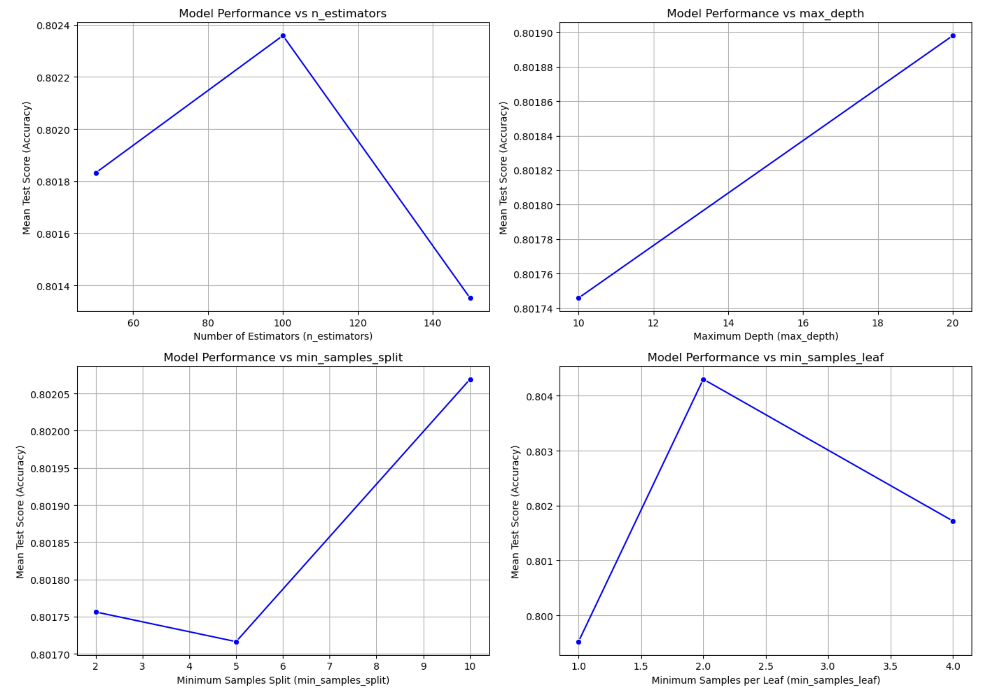
These plots highlight the impact of different hyperparameters on model performance. Parameters like max_depth show consistent improvement in the accuracy, indicating its critical role in enhancing model performance. On the other hand, hyperparameters like n_estimator, min_samples_split and min_samples_leaf exhibit gradual changes upon certain thresholds after which the model performance changes drastically.

Overwhelmed with the amount of information? Discover how to find which hyperparameters matter most with our course Hyperparameter Optimization for Machine Learning.

By observing these trends, we can identify which hyperparameters, like n_estimators and  max_depth, significantly influence model performance. In contrast, parameters like min_samples_leaf and max_features show smaller impact, indicating that they can be safely left “untuned” in time-sensitive scenarios.

Wrapping up

In conclusion, hyperparameter tuning plays a critical role in optimizing machine learning models, and Grid Search provides a powerful, systematic approach to finding the best combination of hyperparameters. Our comparison of the baseline and tuned Random Forest models demonstrated how hyperparameter optimization can substantially improve model accuracy and performance.

While Grid Search is highly effective, it comes with a high computational cost, as it evaluates every possible combination of hyperparameter values, requiring significant time and computational resources. Alternative methods, such as Random Search, offer a more efficient approach by sampling a random subset of the hyperparameter space, significantly reducing computational time while still yielding strong results.

Other models, including Support Vector Machines, Logistic Regression, and XGBoost, also benefit from hyperparameter optimization, making it a key step in enhancing model performance across various machine-learning tasks.

More resources for Hyperparamater Optimization

Master the use of hyperparameters and their tuning techniques with our course Hyperparamater Optimisation in Machine Learning.