Hyperparameters in Machine Learning Explained
Hyperparameters play a critical role in machine learning—they guide how a model learns and directly affect its accuracy and efficiency. Set them well, and performance improves; set them poorly, and results suffer.
In this article, we’ll break down what hyperparameters in machine learning are, why tuning them matters, and explore practical techniques to optimize them. By the end, you’ll understand how even small tweaks can make a big difference in your model’s performance. Let’s get started!
Master hyperparameter optimization with our course Hyperparameter optimization in machine learning.
What are Hyperparameters
Hyperparameters are high-level settings that control how a model learns. Think of them like the dials on an old-school radio—just as you tune a station for clarity, hyperparameters help tune a model for better performance.
Unlike model parameters, which are learned during training, hyperparameters are set before training begins and stay fixed throughout. Choosing the right ones is key to achieving optimal results.
Let’s take a closer look at how hyperparameters differ from parameters.
Parameters vs Hyperparameters
Understanding the distinction between parameters and hyperparameters in machine learning is essential. While they may sound similar, they play very different roles in a model’s learning process.
Let’s understand this with an example. Consider Linear Regression – one of the simplest and most widely used machine learning algorithms. Linear regression aims to find a line that best represents the relationship between input features and the target variable, helping the model predict outcomes for new data based on this relationship. In mathematical terms, a linear regression model aims to find the best-fitting line that predicts the dependent variable y based on the independent variable x.
Here’s the linear regression function:
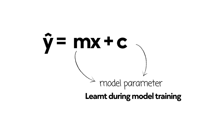
Here m is the slope and c is the intercept of the line. These two variables, m, and c, are the model parameters. These values aren’t set manually. Instead, the model learns them directly from the training data. As the model trains, it adjusts these parameters to minimize the error between its predictions and the actual values. The final values of these parameters determine the position and angle of the line that best fits the data, allowing the model to make accurate predictions (ŷ).
Now, let’s add regularization, which is a common technique to prevent the model from overfitting. When we use regularization in linear regression, we introduce an additional term to the linear regression function (the regularization strength), which discourages the model from fitting too well to the data. This regularization strength (often denoted as λ) is a hyperparameter. This can be seen in the image below:
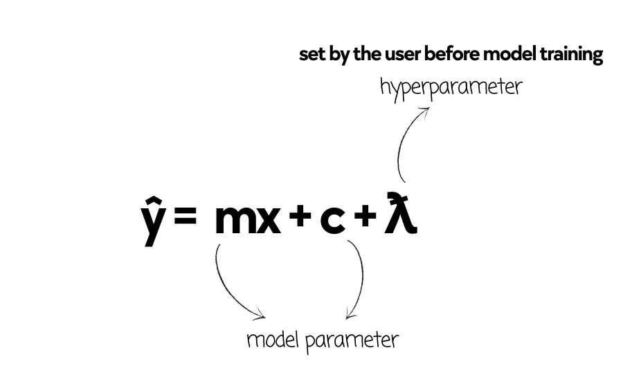
A high regularization value encourages the model to create a simpler, more generalized line, while a low value allows it to fit more closely to the training data. This value of regularization can be adjusted manually to control how the model balances fitting the training data and maintaining generalization based on the problem statement.
In summary, the parameters—intercept and slope—are learned by the model during the training process and cannot be set manually, whereas the hyperparameter—regularization strength—is set manually to control the model’s learning process.
All machine learning models have hyperparameters that can be tuned manually to achieve the desired model performance based on specific goals and data characteristics. Some of the most common hyperparameters in machine learning are the learning rate, regularization strength, maximum depth in tree-based models, kernel type, batch size, and number of iterations.
Ready to tune models like a pro? Our course on Hyperparameter Tuning for Machine Learning will show you how—fast, practical, and hands-on.
Understanding how these hyperparameters affect a machine learning model and its performance can help us select and tune them effectively.
Importance of Hyperparameters
Hyperparameters not only can improve the accuracy of the model, but also play a crucial role in how well a model adapts to new data, how efficiently it trains, and how robust it remains in real-world applications.
A well-tuned model, optimized with carefully selected hyperparameters, can lead to:
1.Better Generalization — Hyperparameters such as the number of layers in a neural network, the number of trees in a random forest, or the degree of a polynomial in a regression model control the complexity of the model and its ability to generalize to unseen data. A model that is too simple tends to underfit, failing to capture the underlying patterns in the data and resulting in poor predictive performance. On the other hand, highly complex models are prone to overfitting, where they capture noise in the training data rather than genuine patterns, leading to misleading predictions when applied to new data. Through thoughtful hyperparameter tuning, such as adjusting regularization strength in linear regression or max depth in decision trees, practitioners can find a balance that allows models to avoid both overfitting and underfitting. This careful calibration results in robust models that not only excel on training data but also yield accurate, dependable predictions in real-world applications. Such improvements in generalization are particularly valuable in fields like healthcare and finance, where predictive accuracy can significantly impact decision-making and outcomes.
2. Improved Training Efficiency — Hyperparameters play a pivotal role in determining how efficiently a model trains, impacting both resource usage and training speed. For instance, adjusting the learning rate in gradient-based algorithms, such as linear regression or support vector machines (SVMs), affects the speed at which the model converges to an optimal solution. A learning rate that is too high can cause the model to overshoot optimal values, while a rate that is too low may lead to excessively long training times. Additionally, hyperparameters like the number of iterations and batch size influence how efficiently a model learns from the training data, directly impacting its training accuracy. A well-balanced choice of hyperparameters allows the model to learn faster without sacrificing accuracy, leading to a machine-learning model that performs effectively on both training and validation datasets. This optimization of training efficiency is crucial in scenarios such as real-time data processing in e-commerce and autonomous vehicles, where timely and accurate predictions can enhance user experience and safety.
3. Improved Interpretability — Hyperparameter tuning can enhance the interpretability of machine learning models, making it easier for data scientists and stakeholders to understand how decisions are made and have transparency and confidence in the outcomes. When hyperparameters are adjusted thoughtfully, they can simplify the model structure, thereby improving the clarity of the relationships between input features and predictions. For instance, in linear regression, the regularization parameter controls the complexity of the model. A well-tuned regularization value can help identify which features are most significant for predictions by shrinking the coefficients of less important features toward zero. This process simplifies the model, making it easier to interpret and understand the relationships between the input variables and the output. Similarly, decision trees benefit from hyperparameter tuning through adjustments like maximum depth and minimum samples per leaf. These changes can create models that are simpler and more straightforward, allowing practitioners to easily communicate insights derived from the model. This is particularly important in fields such as healthcare, finance, and criminal justice, where the implications of model predictions can be significant.
Hyperparameters in Machine Learning
Hyperparameters play a pivotal role in shaping how machine learning models learn, adapt, and perform. Different algorithms come with unique sets of hyperparameters that influence model complexity, training speed, and predictive accuracy.
In this section, we’ll explore some of the most important and widely tuned hyperparameters for various machine learning algorithms. We’ll use Python and scikit learn for code demonstration.
Want to nail hyperparameter optimization with Python? Our course on Hyperparameter Tuning for Machine Learning shows you how—scikit-learn, Hyperopt, Optuna, all frameworks at your fingertips.
Tree Based Algorithms
Tree-based models like Decision Trees, Random Forests, and Gradient Boosting Trees are popular for both classification and regression tasks due to their interpretability and flexibility. The effectiveness of these models often comes from the selection and tuning of key hyperparameters, as they influence the model’s ability to generalize, handle noise, and manage overfitting. Some of the most important and widely tuned hyperparameters for tree-based algorithms are:
-
**Maximum Depth —** defines the deepest level to which a tree can grow. In other words, it limits how many splits each path from the root node can have. When you set a high depth, the tree can split many times, capturing complex patterns but it may lead to overfitting, especially on smaller datasets. Setting a lower depth keeps the model simpler, helping it generalize better but can miss finer details in the data.
from sklearn.tree import DecisionTreeClassifier # Creating a Decision Tree with controlled depth dtc = DecisionTreeClassifier(max_depth=3) dtc.fit(X_train, y_train) -
**Minimum Samples per leaf —**specifies the minimum number of data points required in each leaf node (the final splits). By setting a higher minimum, the model is forced to generalize across larger samples in each leaf, which reduces overfitting. A lower minimum makes the tree more complex, allowing it to capture more patterns at the risk of overfitting.
from sklearn.tree import DecisionTreeRegressor # Decision Tree Regressor with minimum samples per leaf set dtr = DecisionTreeRegressor(min_samples_leaf=10) dtr.fit(X_train, y_train) -
Criterion — decides the quality of a split measuring how “pure” the nodes are. Using “gini” splits the data to minimize impurity, which is often faster. “Entropy,” on the other hand, calculates information gain, which can make more accurate splits but may take longer. For regression, “mse” reduces squared errors to make smoother predictions, while “mae” minimizes absolute errors, which can be better for noisy data.
from sklearn.tree import DecisionTreeClassifier # Using 'entropy' criterion for the classifier dtc = DecisionTreeClassifier(criterion='entropy') dtc.fit(X_train, y_train) -
**Class Weight —** adjusts the importance of each class in classification tasks. This is especially helpful when classes are imbalanced. With “balanced” weights, the model puts more focus on minority classes, improving predictions for these minority classes. Without balanced weights, the model may ignore smaller classes and focus mainly on the majority class, which could affect recall in areas like fraud detection.
from sklearn.ensemble import RandomForestClassifier

# Random Forest with balanced class weights
rf = RandomForestClassifier(class_weight='balanced')
rf.fit(X_train, y_train)
Ensemble Models
Ensemble models, such as Random Forest, AdaBoost, and Gradient Boosting, combine multiple learning algorithms to improve predictive performance over individual models. The tuning of ensemble-specific hyperparameters is essential in achieving optimal model performance, allowing for better control over how each model contributes to the final prediction, the speed of learning, and the overall balance between bias and variance. Key hyperparameters for ensemble models are:
-
Number of Estimators — defines the total number of trees in an ensemble method like Random Forest or XGBoost. Increasing the number of estimators generally boosts model accuracy but increases training time. Fewer trees make the model faster but may reduce its accuracy or stability. Tuning this hyperparameter carefully allows you to balance the model’s performance with the computational cost, especially when working with large datasets or constrained hardware environments.
from sklearn.ensemble import RandomForestClassifier # RandomForest model with a specific number of estimators rf = RandomForestClassifier(n_estimators=100) rf.fit(X_train, y_train) -
Learning Rate — In ensemble models, particularly in boosting algorithms like Gradient Boosting and AdaBoost, the learning rate controls the impact of each weak learner on the final model. A smaller learning rate reduces each learner’s influence preventing any single model from dominating the ensemble. This allows the model to generalize better and avoid overfitting, though it may require more iterations for accuracy. Conversely, a higher learning rate speeds up learning through gradient descent by making larger updates, capturing patterns quickly but risking overfitting. Balancing the learning rate with the number of estimators helps optimize both model accuracy and training efficiency.
from sklearn.ensemble import GradientBoostingClassifier # Gradient Boosting with a specified learning rate gb = GradientBoostingClassifier(learning_rate=0.1, n_estimators=100) gb.fit(X_train, y_train) -
Max Features — refers to the number of features (variables) the model considers when making decisions at each node in bagging algorithms like Random Forest. If you decrease this to a lower value, such as “log2” of the total features, the model becomes more diverse, as each tree sees only a small subset of features. This reduces the chance of overfitting but may lead to slightly less accurate predictions. However, by increasing this to a higher value such as the default “auto” (which is often set to the square root of the total features) the model uses more features to make decisions, which can lead to better performance on training data but might increase the risk of overfitting. Thus, adjusting “max_features” helps control the trade-off between bias and variance in the model.
from sklearn.ensemble import RandomForestClassifier # Random Forest with "sqrt" selected as max_features rf = RandomForestClassifier(max_features='sqrt') rf.fit(X_train, y_train) -
Sub Sample — determines the fraction of the training data that is randomly sampled for training each tree for boosting algorithms like GradientBoost or AdaBoost. It is measured in terms of ratio where a ratio of 1 means using the entire training dataset for each tree, while a value of 0.8 indicates that each tree is trained on only 80% of the training data, randomly sampled without replacement. Adjusting this hyperparameter helps prevent overfitting by introducing randomness and reducing the correlation between trees.
from sklearn.ensemble import GradientBoostingClassifier

# Gradient Boosting using 80% of data for each estimator
gbc = GradientBoostingClassifier(subsample=0.8)
gbc.fit(X_train, y_train)
Linear Models
Linear models, including Linear Regression, Logistic Regression, and Support Vector Machine, among others, rely on specific hyperparameters to control aspects such as regularization, optimization, and decision boundary complexity. These models often work well when data is linearly separable or close to it. Hyperparameters play a crucial part in optimizing how a linear model performs. Some of the most commonly tuned hyperparameters for linear models are:
-
Regularisation (C) — prevents overfitting by adding a penalty term to the loss function, thereby controlling the model’s complexity. Regularization is of two types – L1 (Lasso) and L2 (Ridge). L1 regularization penalizes coefficients to zero for feature selection, while L2 reduces them for stability. Increasing the regularization strength penalizes the model more and thus reduces model complexity by shrinking coefficients. Reducing the regularization strength allows more flexibility, making the model fit more closely to the training data, which may increase overfitting. “C” is generally represented as the reverse of regularization strength.
from sklearn.linear_model import LogisticRegression # Applying a lower C for increased regularization model = LogisticRegression(C=0.5) -
Fit Intercept — determines whether the model should calculate an intercept term. Setting “fit_intercept” as True allows the model to fit an intercept term, shifting the line to better fit the data. If set to False, the model assumes data is centered at the origin, which may lead to poor performance if the data is not zero-centered.
from sklearn.linear_model import LinearRegression # Allows the model to adjust the intercept model = LinearRegression(fit_intercept=True) -
Solver — specifies the optimization algorithm used to minimize the cost function in models like Logistic Regression. Different solvers can impact the speed and convergence of model training. For instance, ‘liblinear’ works well with small datasets, while ‘saga’ supports both L1 and L2 penalties and is more efficient for larger datasets. Choosing the right solver helps improve training speed without compromising on accuracy.
from sklearn.linear_model import LogisticRegression

# "liblinear" solver suited for smaller datasets
model = LogisticRegression(solver='liblinear')
Clustering Models
Clustering models, like K-Means and Hierarchical Clustering, use a set of hyperparameters that influence how clusters are formed, helping the model identify natural groupings within a dataset. Fine-tuning these hyperparameters can significantly impact the clustering quality and efficiency, especially on large or complex datasets. Here are some essential hyperparameters for clustering models:
-
Number of Clusters — determines how many groups the algorithm should divide the data into. Increasing the number of clusters creates more, smaller groups, potentially capturing subtle patterns in the data, while fewer clusters create larger, more generalized groups. The choice of “n_clusters” should balance model interpretability with capturing data variation effectively.
from sklearn.cluster import KMeans # 5 clusters to segment the data model = KMeans(n_clusters=5) -
Distance Metric — defines how distances between data points are measured, which impacts how clusters are formed. Common metrics include Euclidean, Manhattan, and Cosine distances. Euclidean distance focuses on straight-line distances, making it sensitive to scale, whereas Cosine distance focuses on the angle, which is useful for high-dimensional or text data. The choice of distance metric can impact the shape and size of clusters, especially in Hierarchical Clustering.
from sklearn.cluster import AgglomerativeClustering # Using Cosine distance model = AgglomerativeClustering(distance_threshold=None, n_clusters=3, affinity='cosine') -
Maximum Iterations — limits how many times the algorithm refines clusters to reach a stable solution. More iterations allow for fine adjustments, which may lead to better-defined clusters, but can increase computational time. Reducing it speeds up the algorithm but might result in less stable clusters if the data is complex.
from sklearn.cluster import KMeans

# Allows more iterations for better convergence
model = KMeans(n_clusters=3, max_iter=300)
Other machine learning models
In addition to the models we’ve covered, other popular machine learning algorithms come with essential hyperparameters that impact their performance.
Support Vector Machines (SVM) use hyperparameters like kernel type for modeling non-linear data, while Naive Bayes includes options such as smoothing for managing zero probabilities in categorical data.
Deep learning models like neural networks involve hyperparameters such as the number of hidden layers, which determines the network’s depth and influences how neurons capture complex patterns, or the activation function, which dictates how to integrate the outputs of neurons from former layers. In addition, epochs, dropout rate, and batch size, influence training duration, model complexity, and the accuracy of the model.
All these hyperparameters, when tuned carefully, enhance each model’s ability to perform effectively across diverse data scenarios. This makes model hyperparameter tuning a critical process for professionals spanning across various fields where data science applications drive critical insights.
Hyperparameter Tuning Techniques
Hyperparameter optimization plays a critical role in improving the performance of machine learning models. By fine-tuning hyperparameters, you can significantly enhance a model’s ability to generalize to new data, ensuring it performs well in diverse scenarios. Depending on the problem’s complexity and the number of hyperparameters involved, different tuning techniques can be applied to efficiently find the optimal hyperparameters. Common methods like Grid Search, Random Search, and Bayesian Optimization offer distinct advantages and challenges when it comes to exploring combinations of hyperparameters for different models. These techniques are designed to help data scientists identify the best configuration that maximizes a model’s performance.
Grid search
Grid Search is a straightforward and exhaustive technique used for hyperparameter optimization. It involves specifying a grid of different hyperparameters and evaluating all possible combinations of these values. For each combination, the model is trained and validated using cross-validation to determine the best-performing set of hyperparameters based on their score. The score is typically the average of the cross-validation scores, such as accuracy for classification tasks or mean squared error for regression.
For example, if you are tuning a random forest model, you might define a grid with different values for n_estimators (e.g., 50, 100, 200) and max_depth (e.g., 10, 20, 30). Grid Search will then evaluate all possible combinations of these values to identify the best one for the model.
Here’s how the best hyperparameters can be found using Grid Search in Python:
from sklearn.model_selection import GridSearchCV
from sklearn.ensemble import RandomForestClassifier

# Initialize the model
model = RandomForestClassifier()

# Define the parameter grid
param_grid = {
    'n_estimators': [50, 100, 200],  # Number of trees in the forest
    'max_depth': [None, 10, 20],  # Depth of each tree
    'min_samples_split': [2, 5, 10]  # Minimum samples required to split an internal node
}

# Set up GridSearchCV with cross-validation
grid_search = GridSearchCV(estimator=model, param_grid=param_grid, cv=5, scoring='accuracy')

# Fit Grid Search to the data
grid_search.fit(X_train, y_train)

# Output the best hyperparameters and score
print("Best Hyperparameters:", grid_search.best_params_)
print("Best Score:", grid_search.best_score_)
# SAMPLE OUTPUT
Best Hyperparameters: {'max_depth': 20, 'n_estimators': 200, 'min_samples_split': 2}
Best Score: 0.934
Grid Search can be computationally expensive as it requires evaluating every combination, especially when the number of possible combinations is large. Therefore, Grid Search is particularly effective when you have a relatively small set of hyperparameters to tune and want to ensure you explore every possible combination to find the most suitable one for your model.
Master the use of the different hyperparameter optimization strategies with our course Hyperparamater Optimization in Machine Learning
Random Search
Random Search is a more efficient technique for hyperparameter optimization compared to Grid Search, especially when dealing with a large search space. Unlike Grid Search, which exhaustively evaluates every possible combination of hyperparameter values, Random Search randomly selects combination of hyperparameter and evaluates them. In Random Search, the number of combinations is not pre-defined but is based on how many iterations you want to perform. Each iteration involves randomly selecting values for a subset of hyperparameters and evaluating the model’s performance using cross-validation. By repeating this process multiple times, Random Search can find good (if not the best) hyperparameter combinations much faster than Grid Search.
Here’s how the best hyperparameters can be found using Random Search in Python:
from sklearn.model_selection import RandomizedSearchCV
from sklearn.ensemble import RandomForestClassifier
from scipy.stats import randint

# Initialize the model
rf = RandomForestClassifier()

# Define the hyperparameter grid to sample from
param_set = {
    'n_estimators': randint(50, 200),
    'max_depth': randint(10, 50),
    'min_samples_split': randint(2, 20),
    'min_samples_leaf': randint(1, 20)
}

# Set up the RandomizedSearchCV
random_search = RandomizedSearchCV(rf, param_distributions=param_set, n_iter=100, cv=5, n_jobs=-1, random_state=42)

# Fit the model to the data
random_search.fit(X_train, y_train)

# Output the best parameters and score
print("Best Hyperparameters:", random_search.best_params_)
print("Best Score:", random_search.best_score_)
# SAMPLE OUTPUT
Best Hyperparameters: {'max_depth': 25, 'min_samples_leaf': 6, 'min_samples_split': 15, 'n_estimators': 150}
Best Score: 0.935
In the previous code, we have set n_iter to 100, which means 100 random combinations of the hyperparamaters will be evaluated.
Random Search is best used when dealing with a large hyperparameter space or when time is limited. It efficiently explores random combinations of hyperparameters, making it ideal for situations where you want to quickly identify good parameter values without exhaustively testing every possible combination. It’s particularly useful when you’re unsure of the optimal values and want to cover a broad range with fewer iterations.
Bayesian optimization
Bayesian Optimization is a smart and efficient way to find the best hyperparameters for a model. It is a probabilistic model-based technique working on the principle of Bayes’ Theorem, which updates the probability of a hypothesis based on new evidence. Unlike Grid Search and Random Search, which test combinations of hyperparameters randomly or exhaustively, Bayesian Optimization tries to predict which hyperparameters are likely to give the best results based on past tests. It intelligently explores the hyperparameter space by balancing exploration (trying new, untested areas) and exploitation (focusing on areas known to work well), allowing it to converge on optimal hyperparameters more efficiently.
Here’s how how the best hyperparameters can be found using Bayesian optimization in Python:
from skopt import BayesSearchCV
from sklearn.ensemble import RandomForestClassifier

# Initialize the model
model = RandomForestClassifier()

# Define the search space for hyperparameters
param_space = {
    'n_estimators': (50, 200),  # Number of trees in the forest
    'max_depth': (3, 20),        # Maximum depth of trees
    'min_samples_split': (2, 10) # Minimum samples to split a node
}

# Set up Bayesian Optimization
opt = BayesSearchCV(model, param_space, n_iter=30, cv=5, n_jobs=-1)

# Fit the model with the optimized hyperparameters
opt.fit(X_train, y_train)

# Print the best hyperparameters found
print("Best hyperparameters:", opt.best_params_)
# SAMPLE OUTPUT
Best hyperparameters: {'max_depth': 18, 'min_samples_split': 4, 'n_estimators': 150}
Bayesian Optimization is ideal when you have a complex hyperparameter space and need to maximize efficiency in finding the optimal values, as it minimizes the number of model trainings needed to find the best hyperparameters. It’s particularly valuable for tuning models that are computationally expensive to train, such as deep learning models or large ensemble methods where other search methods might be too slow or ineffective.
Wrapping up
In conclusion, hyperparameters are crucial to optimizing the performance of machine learning models, directly influencing the model architecture and its ability to learn effectively. By carefully selecting and tuning these parameters, we can significantly improve the model’s ability to generalize to new data, avoid overfitting, and optimize computational efficiency. Whether you are working with tree-based algorithms, linear models, or deep learning, understanding the impact of different hyperparameters is essential. The techniques for hyperparameter tuning, including grid search, random search, and Bayesian optimization, provide a range of strategies to find the optimal settings for your model. With the right combination of hyperparameters, you can enhance model performance and unlock more accurate, reliable predictions for real-world applications.
More resources for Hyperparamater Optimization
Master the use of hyperparameters and the different optimization strategies with our course Hyperparamater Optimization in Machine Learning