How to Detect Outliers in Python: A Comprehensive Guide

Real-world data science datasets often contain anomalies and errors that hide true patterns and make accurate conclusions difficult. Outliers are key among these—data points that stand apart due to errors, natural variation, or rare but valid conditions.

Handling outliers is a crucial skill, as they can distort analysis, skew predictions, and mislead decisions. Managing them well leads to cleaner data and clearer insights.

In this article, we’ll explore how to detect outliers in Python—using plots, statistical techniques, and machine learning. Then, we’ll apply these methods step-by-step on a real dataset.

To learn more about detecting and handling outliers in Python, check out our course Feature Engineering for Machine Learning.

Let’s dive in.

What Are Outliers?

Outliers are data points that differ significantly from the rest of the dataset. In statistical terms, outliers are values that are far away from the average or the expected range of the data.

For instance, if you are analyzing the heights of a group of people and most heights range from 150 to 190 cm, a height of 250 cm would be an outlier. Similarly, a height of 80 cm would also be an outlier. Here is an example to illustrate this :

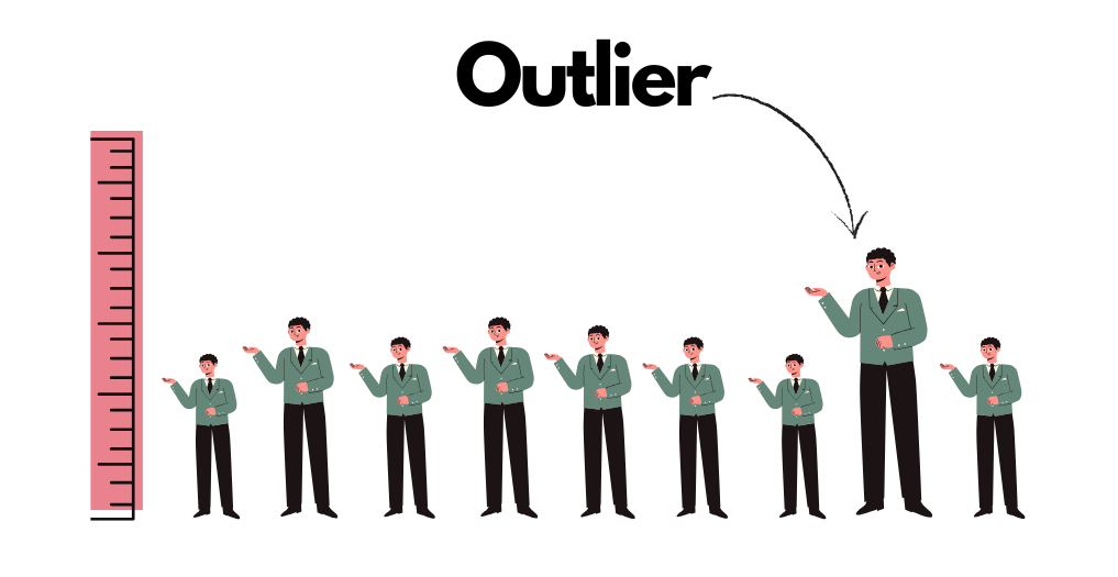
In real-world datasets, outliers can arise due to various reasons which can be categorized as follows:

• Human Errors: Data entry errors, experimental errors while data extraction, or intentional errors to test detection algorithms, among others.
• Data Processing Errors: Data manipulation errors or sampling errors.
• Instrument Errors: Measurement errors that occur due to faulty instruments while collecting data.
• Natural Outliers: Genuine anomalies that are not errors but represent rare events in the data.

Types of Outliers

Understanding the different types of outliers is essential for effective detection and analysis. Outliers can be categorized based on their characteristics and how they relate to the rest of the data. Here are the main types:

1. Univariate Outliers: These occur when a single data point significantly deviates from the rest for one variable. For example, a student scoring 20 in a dataset where most scores range from 60 to 90 is a univariate outlier.
2. Multivariate Outliers: These arise when multiple variables are considered. For instance, a house priced at $700,000 with a size of 1,500 square feet, while most similar houses are priced between $250,000 and $350,000 and range from 1,800 to 2,200 square feet, is a multivariate outlier.
3. Contextual Outliers: These are unusual given specific conditions. For example, a temperature of 100°F is normal in summer but a contextual outlier in winter.
4. Collective Outliers: These consist of groups of data points that behave differently from the norm. For instance, a clothing store selling 1,000 items each day over three days during Black Friday is a collective outlier

Now that we know the different types of outliers, it’s essential to consider how they can impact our data. Outliers can skew results and lead to inaccurate conclusions, making it important to understand their effects.

Impact of Outliers on Data

Outliers can significantly skew statistical analyses and model predictions. They can affect measures of central tendency such as the mean and measures of variability such as the standard deviation, leading to distorted insights. Let’s delve a little deeper into the impact of outliers.

Impact on Measures of Central Tendency

The central tendency of a dataset represents the center or typical value of the data. The three main measures of central tendency are the mean, median, and mode. Let’s see how outliers influence these measures.

Mean

The mean, or average, is the most commonly used measure of central tendency. The mean is highly sensitive to extreme values. An outlier, whether it is very high or very low, can pull the mean away from the true central tendency of the data.

For example, consider a dataset of exam scores: [85, 87, 90, 92, 95, 100, 150]. In this case, the score of 150 acts as an outlier, pulling the mean away from the actual performance of most students.

Mean : 99.85

The mean of 99.85 suggests that students performed exceptionally well. However, most scores cluster between 85 and 100. The outlier of 150 skews the mean upward, creating a misleading conclusion about the overall performance.

While the mean can be skewed by outliers, other measures like the median and mode provide a more stable view of the central tendency as they do not rely on every data point.

Impact on Measures of Variability

Measures of variability describe how spread out or dispersed the values in a dataset are. The most common measures of variability include the range, variance, and standard deviation. Here’s how outliers affect these measures.

Range

The range is the simplest measure of variability, calculated as the difference between the maximum and minimum values in a dataset. While the range gives a quick idea of how spread out the data is, outliers can inflate it, making the data seem more varied than it truly is.

For example, consider the dataset: [10, 12, 15, 14, 11, 200]. We can calculate the range as:

Range: 200 – 10 = 190

This large range of 190 suggests a huge spread in the data, but most values cluster closely together between 10 and 15. The outlier 200 inflates the range. This can lead analysts to believe there’s more variation than there actually is, which may affect decision-making or further analysis.

Variance and Standard Deviation

The variance measures how much each number in a dataset differs from the mean, indicating how spread out the data is. The standard deviation is simply the square root of the variance and provides a measure of this spread in the same scale as the value range.

For our data : [10, 12, 15, 14, 11, 200], the variance and standard deviation would be:

Mean: 43.67 Variance: 4890.89 Standard Deviation: 69.93

The variance and standard deviation are inflated due to the outlier (200). While most values are closely grouped, the outlier makes the dataset appear more varied than it is.

Standard deviation is less affected by outliers than the variance, because the variance squares the difference between the mean and the outliers.

Impact on Statistical Tests and Models

Outliers can significantly distort the results of statistical tests and machine learning models. Since many models and tests rely on assumptions about the data distribution, extreme values can mislead both analysis and predictions, making it crucial to detect and handle outliers properly before analysis.

Statistical Tests

Outliers can disrupt the assumptions of statistical tests, such as t-test, ANOVA, or correlation, and their impact can be broken down as follows:

• Violation of Normality Assumption: Most statistical tests assume that the data follows a normal distribution. Outliers can distort this distribution, leading to inaccurate p-values and confidence intervals, which can lead to incorrect decisions regarding hypotheses.
• Inflated Correlation Coefficients: In correlation tests, outliers can artificially increase (or decrease) the correlation between variables. For instance, the presence of extreme values in a dataset might create a misleadingly strong correlation where none exists.

Imagine a dataset tracking students’ study hours and their exam scores. Most students study between 5 and 15 hours, scoring between 70 and 90. However, one student studied for 50 hours and scored 100. This student is an outlier. Because of this extreme value, the correlation between study hours and exam scores may appear stronger than it truly is. It could mislead educators into believing that studying significantly longer guarantees higher scores, while most students achieve good results with typical study hours.

Regression Models

Outliers can significantly distort regression models, especially linear regression. The presence of extreme values in the data can pull the regression line toward the outliers, reducing the model’s ability to capture the true relationship between variables. Key impacts include:

• Skewed Slope: Outliers affect the slope of the regression line, which may result in overestimated or underestimated predictions for the rest of the dataset.
• Poor Predictions: When the regression line is pulled toward outliers, the model’s overall accuracy decreases, leading to unreliable predictions for future data points.

Consider a dataset predicting house prices based on size in square feet. Most houses are priced between $150,000 and $500,000, and one house with 10,000 sq ft is priced at $1,500,000. This house is an outlier and can skew the regression line. Instead of showing a steady increase in price with size, the line is pulled upward, suggesting that even a small increase in size dramatically raises the price. Consequently, when predicting the price of a 2,000 sq ft house, the model might incorrectly estimate it at $600,000 instead of the more accurate $400,000.

Machine Learning Algorithms

Outliers can affect machine learning algorithms in various ways, depending on the algorithm’s sensitivity to extreme values:

• Sensitive Algorithms: Algorithms such as Linear Regression, K-means clustering, and Support Vector Machines (SVM) are highly sensitive to outliers. For example, in K-means clustering, an outlier can pull the centroid toward it, resulting in clusters that misrepresent the true data distribution.
• Robust Algorithms: Algorithms like Decision Trees and Random Forests are robust to outliers, minimizing their influence for more reliable predictions.

In summary, outliers can have a far-reaching impact on the reliability of statistical tests, machine learning models, measures of central tendency, and variability. Sensitive algorithms are particularly vulnerable, leading to unreliable predictions, while robust algorithms can mitigate some of their impact.

Therefore, to ensure accurate analysis and optimal model performance, it is crucial to detect and handle outliers effectively in our data. Various techniques allow you to detect outliers, ranging from simple visualizations to the application of machine learning models.

Methods for Outlier Detection

When it comes to outlier detection, there isn’t a one-size-fits-all solution. Different datasets and problems may require different approaches.

In this section, we’ll walk you through several techniques used to detect outliers in Python—starting with visual methods and progressing to more advanced statistical and algorithmic approaches. We will use the California Housing Dataset from sklearn, along with the Python library Feature-engine to detect outliers.

To master outlier detection in Python and take your skills further, enroll in our course Feature Engineering for Machine Learning.

Let’s start by importing libraries and loading and preprocessing the dataset for outlier detection.

import pandas as pd
import numpy as np
import matplotlib.pyplot as plt
import seaborn as sns
from sklearn.datasets import fetch_california_housing
from feature_engine.outliers import OutlierTrimmer
from sklearn.model_selection import train_test_split

# Loading the California Housing Dataset
c = fetch_california_housing()
data = pd.DataFrame(california_housing.data, columns=california_housing.feature_names)

# Adding the target column (median house value)
data['MedianHousePrice'] = california_housing.target

# Rounding off every value to 2 decimal places for easy view.
data = data.round(2)

# Display the first few rows of the dataset
data.head()

In the following image, we see the California housing dataset:

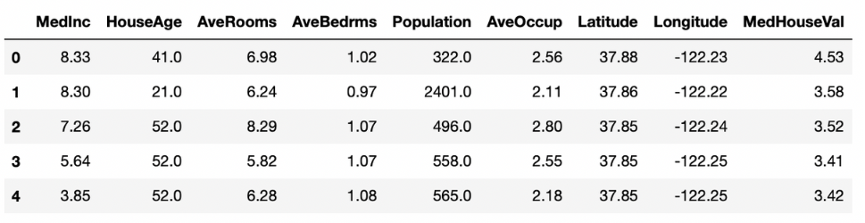
Here’s a representation of the dataset features:

MedInc: Median income of households in the block group (in tens of thousands of dollars). HouseAge: Median age of the houses within the block group. AveRooms: Average number of rooms per household. AveBedrms: Average number of bedrooms per household. Population: Total population in the block group. AveOccup: Average number of occupants per household. Latitude: Latitude of the block group. Longitude: Longitude of the block group. MedHouseVal: Median house value in the block group (in hundreds of thousands of dollars)

Now that we have the dataset ready, let’s dive into the outlier detection techniques.

Visualization Techniques

Visualizing data is often the simplest and most intuitive way to spot outliers. Common plots include boxplots, scatter plots, and histograms, which help visually detect extreme values.

# ---- Boxplot ----
# Boxplot for Median House Value
plt.figure(figsize=(8, 6))
sns.boxplot(x=data['Population'])
plt.title('Boxplot for Population')
plt.show()

# ---- Scatterplot ----
# Scatterplot for Median Income vs Median House Value
plt.figure(figsize=(8, 6))
sns.regplot(x=data['AveRooms'], y=data['AveBedrms'], scatter_kws={'alpha':0.5}, line_kws={"color":"darkblue"})
plt.title('Scatter Plot - Average #Rooms vs Average #Bedrooms with Regression Line')
plt.xlabel('Average Number of Rooms')
plt.ylabel('Average Number of Bedrooms')
plt.show()

# ---- Histogram ----
# Histogram for Average Rooms
plt.figure(figsize=(8, 6))
sns.histplot(data['MedInc'], bins=50, kde=True)
plt.title('Histogram for Median Income')
plt.show()

Below is the output of the code block:

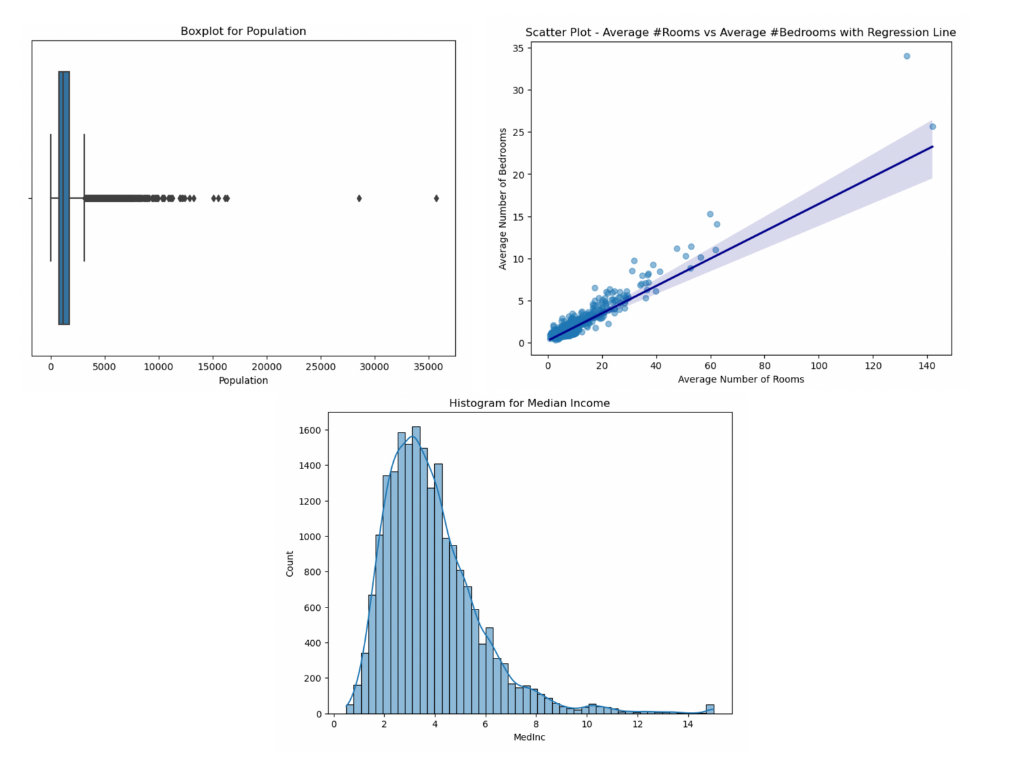
In the boxplot, points beyond the whiskers are considered outliers. The scatter plot offers insights into the relationship between the two features, and outliers often stand out as points far from the general trend line. A histogram provides a visual representation of the distribution of values within a single feature, where outliers are typically represented as bars that are distant from the main cluster of data.

While visualizations effectively highlight potential outliers, statistical techniques provide a more objective approach to detecting these anomalies in our dataset

Statistical Techniques

Statistical techniques help us quantify outliers based on certain metrics, making it easier to set thresholds for detection. Some popular methods include:

Z-Score method

The Z-Score method standardizes data and finds how far a data point is from the mean in terms of standard deviations. It helps us identify outliers by showing which points are significantly higher or lower than most others. The Z-Score is calculated as:

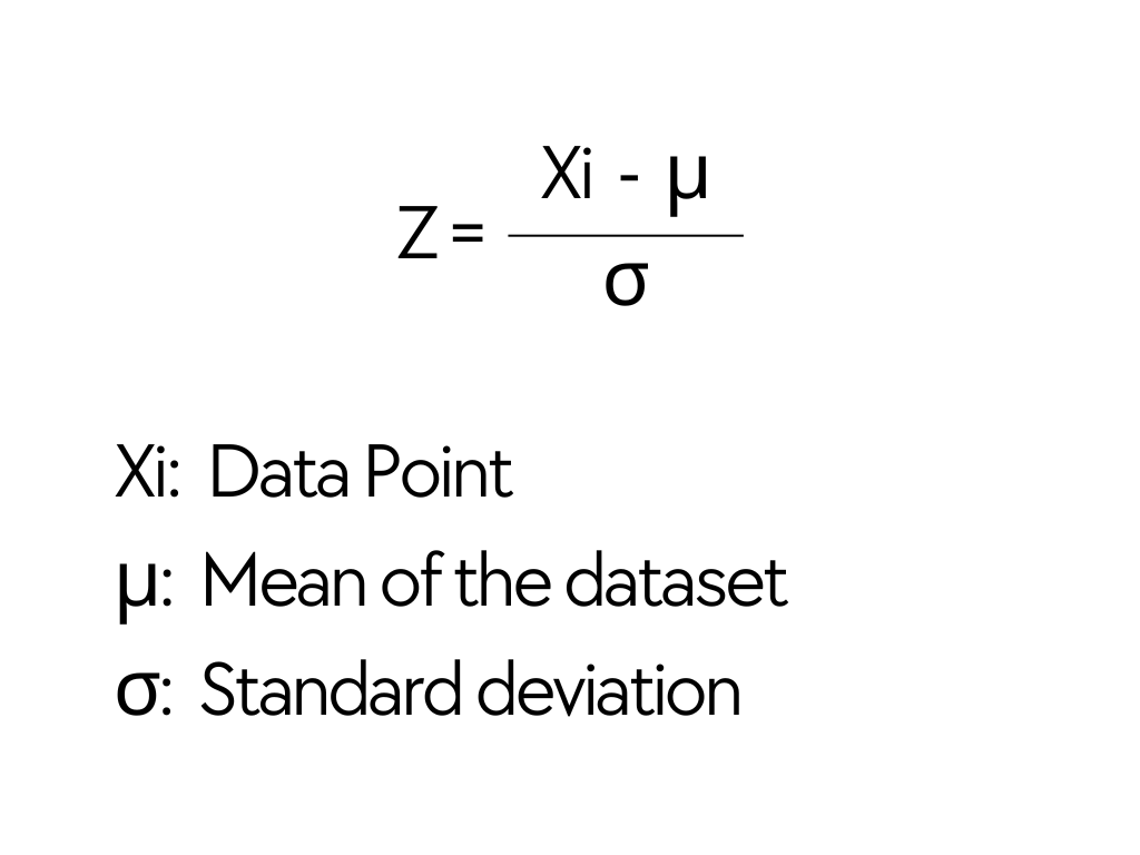
A Z-score greater than 3 or less than -3 is often considered an outlier. It indicates that a point is 3 standard deviations away from the mean.

# Calculate mean and standard deviation for the 'MedInc' column
mean_medinc = data['MedInc'].mean()
std_medinc = data['MedInc'].std()

# Calculate Z-scores for the 'MedInc' column
z_scores = (data['MedInc'] - mean_medinc) / std_medinc

# Identify data points where the Z-score is greater than 3 or less than -3
outliers_zscore = data[abs(z_scores) > 3]

# Display the outliers
# outliers_zscore.head()

#See the number of outliers
print("Number of outliers detected by Zscore: ",outliers_zscore.shape[0])

Below is the output of the previous code block:

Number of outliers detected by Zscore: 345

IQR method (Interquartile Range Proximity Rule)

The IQR method calculates the range between the first quartile (25th percentile) and the third quartile (75th percentile). It helps identify outliers by setting boundaries.

To determine these boundaries, we look at how far the data points are from the middle. Typically, the points that are 1.5 times the IQR below the first quartile or above the third quartile are considered outliers.

This means that if a value is too far from the main group of data points, it will be marked as an outlier. We can directly do this in Python using the quantile method:

# Calculate IQR
Q1 = data['MedInc'].quantile(0.25)
Q3 = data['MedInc'].quantile(0.75)
IQR = Q3 - Q1

#Calculate the boundaries - lower and upper
lower_bound = Q1 - 1.5 * IQR
upper_bound = Q3 + 1.5 * IQR

#Find Outliers - points above or below the boundaries
iqr_outliers = data[(data['MedInc'] < lower_bound) | (data['MedInc'] > upper_bound)]

# Display the outliers
# iqr_outliers.head()

#See the number of outliers
print("Number of outliers detected by IQR method: ", iqr_outliers.shape[0])

The following is the output of the previous code:

Number of outliers detected by IQR method: 679

Want to have these code recipes packed nicely in a book? Check out our Python Feature Engineering Cookbook.

Statistical techniques are robust and provide a solid foundation for identifying outliers. However, in complex datasets where multiple variables interact, more sophisticated approaches like algorithmic techniques for outlier detection are often used.

Algorithmic Techniques

Algorithmic techniques use machine learning and clustering methods to detect outliers, making them suitable for complex datasets with multiple features. Two of the most widely used algorithmic techniques for outlier detection are Isolation Forests and Local Outlier Factor (LOF).

Isolation Forests

Isolation Forest is an ensemble learning method specifically designed for anomaly detection. It works by building a collection of decision trees, where each tree separates the data points based on random features and random values of those features. The main idea is that outliers, or unusual points, can be isolated more easily than regular data points. As the trees split the data, each point is assigned to a node, and outliers will generally reach the leaf nodes more quickly because they are far away from the normal clusters of data. The fewer splits it takes to isolate a point, the more likely it is to be an outlier. Each point gets an anomaly score—lower scores indicate potential outliers.

When we compare Isolation Forest to other methods like Random Forest, we see some key differences. Random Forest is mainly used for classifying data and combines many trees for better accuracy. In contrast, Isolation Forest focuses solely on identifying outliers quickly and effectively. By examining how deep into the tree a data point goes before reaching a leaf node, we can determine if it is an outlier. This makes it a great choice for spotting unusual patterns in data.

In practice, the Isolation Forest algorithm identifies outliers based on the characteristics of the entire dataset. It assigns an outlier flag to each data point, where -1 indicates an outlier and 1 indicates an inlier.

Let’s fit an Isolation Forest model to our entire dataset and then flag the outliers:

from sklearn.ensemble import IsolationForest

# Fit the Isolation Forest model with a contamination rate (expected outlier ratio)
isolation_forest = IsolationForest(contamination=0.01)

# Use the model to predict outliers (-1) and inliers (1)
outliers_if = isolation_forest.fit_predict(data)

# Append the outlier flag to the dataset
data['Outlier'] = outliers_if

# Filter and display identified outliers
outliers_If = data[data['Outlier'] == -1]
print("Number of outliers detected by Isolation Forests:", outliers_If.shape[0])

Below is the output of the previous code block:

Number of outliers detected by Isolation Forests: 207

Once we identify the outliers, we can visualize their relationships by plotting any two variables. The scatter plot illustrates how the Isolation Forest algorithm highlights anomalies based on the interaction between these features:

# Visualize the results
plt.figure(figsize=(8, 6))
plt.scatter(x=data['MedHouseVal'], y=data['AveRooms'], c=data['Outlier'], cmap='coolwarm', s=50)
plt.title('Isolation Forest - Outlier Detection')
plt.xlabel('Median House Value (in $10k)')
plt.ylabel('Average Number of Rooms')
plt.show()

The following image results from the previous code block:

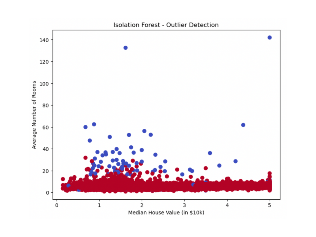
The contamination parameter in the Isolation Forest specifies the expected proportion of outliers in the data. By setting contamination = 0.05, we indicate that we expect approximately 5% of the data points to be outliers. If it’s set too low, the model may not flag many points as outliers.

Local outlier Factor (LOF)

Local Outlier Factor (LOF) is a method used to identify outliers based on how different a data point is from its neighbors. Unlike some other techniques that look at the entire dataset, LOF focuses on the local area around each data point. This means that it can find outliers even in datasets where points are packed together at different densities.

In simpler terms, LOF checks how crowded an area is. If a point is in a sparsely populated region compared to its neighbors, it gets marked as an outlier. This makes LOF especially useful for datasets where data points can be clustered in various ways.

Similar to Isolation Forests, LOF assigns an outlier flag to each data point, where -1 indicates an outlier and 1 indicates an inlier. We can then plot the identified outliers using a scatterplot.

Here’s how we can use LOF in Python:

from sklearn.neighbors import LocalOutlierFactor

# Initialize LOF model
lof = LocalOutlierFactor(n_neighbors=20)

# Fit the model and predict outliers
data['Outlier'] = lof.fit_predict(data)
outliers_Lof = data[data["Outlier"] == -1]
print("Number of outliers detected by LOF:", outliers_Lof.shape[0])

Below is the output of the previous code block:

Number of outliers detected by LOF: 166

We can plot the outliers between any two variables as follows:

plt.figure(figsize=(8, 6))

# Scatter plot for visualization
plt.scatter(data['MedHouseVal'], data['AveRooms'],
            c=data['Outlier'], cmap='coolwarm', s=100, edgecolor='k')

# Highlight the outliers
plt.scatter(outliers_Lof['MedHouseVal'], outliers_Lof['AveRooms'],
            color='red', s=200, label='Outliers', edgecolor='black')

# Labels and title
plt.title('Local Outlier Factor (LOF) Outlier Detection')
plt.xlabel('MedHouseVal')
plt.ylabel('AveRooms')
plt.axhline(y=250000, color='r', linestyle='--', label='Price Threshold')
plt.axvline(x=4, color='g', linestyle='--', label='Room Threshold')
plt.legend()
plt.grid()
plt.show()

The following image results from the previous code block:

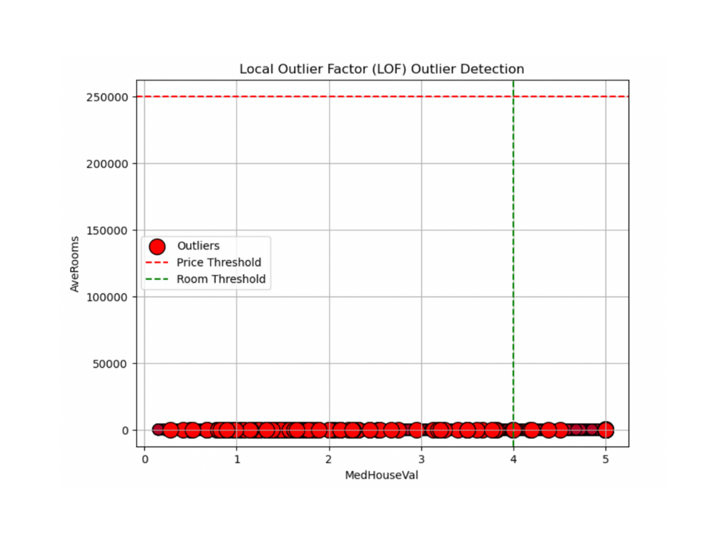
The n_neighbors parameter in the LOF algorithm defines how many neighboring points to consider for calculating the density. The threshold values on the scatterplot indicate that the data points significantly above this value might be considered outliers in the context of the dataset.

Both these outlier detection methods are highly effective in complex, feature-rich datasets where basic visualization and statistical methods might fall short.

Now that we’ve explored various techniques for outlier detection, it’s essential to understand how to effectively handle these outliers to improve the accuracy and reliability of our data analysis.

Handling Outliers

Once you have identified the outliers in our dataset, it’s essential to handle these outliers with a dedicated strategy that aligns with your analysis goals. In general, we can remove or cap outlier values.

Removing Outliers

Removing outliers involves deleting the rows with outliers from the dataset. While this approach can help improve model accuracy, it risks losing valuable information. This technique can be used when outliers are clearly erroneous or are present due to data entry mistakes. For example—negative values for house prices.

Following from our previous code examples, this is how we can remove the outliers from the data:

# Remove outliers from the dataset
clean_data = data[data['Outlier'] != -1]

Capping

Capping involves replacing extreme values in the dataset with specified maximum values. These maximum values can be determined using the z-score, the IQR rule or percentiles.

By capping outliers, we keep all the data while reducing the effect of outliers. This technique can be used to maintain the overall quality of your dataset but need to lessen the impact of extreme values. For instance, very high sales figures in sales data can distort the analysis, and capping helps ensure your results are more accurate.

Feature-engine, is a python open source library that supports removing or capping outliers by using transformers that work exactly like those from scikit-learn. With the method fit(), the transformer finds the boundaries beyond which a value will be considered an outlier, and with transform() they either cap or remove the outliers.

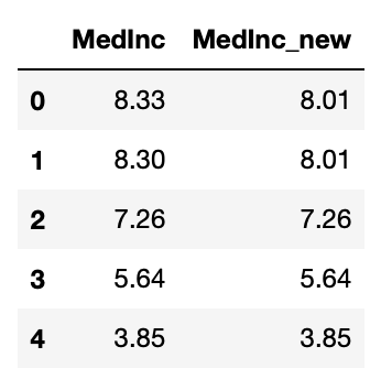
In the following code block, I use Winsorizer from Feature-engine to cap outliers, which are identified as those values beyond the 1st or 3rd quartile plus 1.5 the IQR:

import numpy as np
import pandas as pd
from feature_engine.outliers import Winsorizer
X = data[['MedInc']]
wz = Winsorizer(capping_method='iqr')
X['MedInc_new'] = wz.fit_transform(X)
X.head()

Below, we se the transformed dataframe:

And that’s a wrap!

More resources to detect outliers in Python

For more details and Python code to detect and remove or cap outliers, check out our Python Feature Engineering Cookbook:

For video tutorials and Python implementations, check out our course Feature Engineering for machine learning: