Missing data is a common challenge in machine learning and statistical analysis, and handling it appropriately is crucial for obtaining valid inferences. One of the simplest approaches to dealing with missing data is Complete Case Analysis (CCA), also known as listwise deletion.

In this article, we’ll deep dive into CCA, including:

• The CCA concept
• Missing data mechanisms
• CCA advantages and limitations
• Other potential ways to deal with missing data
• Hands-on Python examples showcasing CCA in distinct scenarios

We’ll use simulated datasets and Python functions to illustrate how CCA works in distinct scenarios.

Want to go beyond the theory and see CCA (and other missing data imputation methods) in action? Check out our course on Feature Engineering for Machine Learning, where we cover practical implementations with Python and real datasets.

Without further ado, let’s get started!

What is Complete Case Analysis?

Complete Case Analysis (CCA) is a method for handling missing data by excluding any rows (cases) with missing values in any of the variables of interest. In other words, only the cases with complete data are used for analysis (therefore, “complete case analysis”). This approach is straightforward to implement, but it has some limitations that we’ll discuss in the article.

How to apply it?

Let’s say we have a pandas dataframe called df. We can call df.dropna() to drop all rows with missing values, and here we go! That’s it, that’s simple! We’ve created a dataset for complete case analysis that we can use to train our machine-learning models! Very straightforward, right?!

However, as mentioned, it has some limitations, and knowing when it would not be appropriate is essential. To understand its limitations, we must first understand the missing data mechanisms.

You can also apply CCA by using the class DropMissingData from Feature-engine (see section “CCA Pipeline with Feature-engine”).

Understanding Missing Data Mechanisms

There are three primary missing data mechanisms as defined by Rubin:

1. Missing Completely at Random (MCAR): The probability of a missing value being independent of both observed and unobserved data. The “missingness” is purely random.
   • Example: A survey respondent forgets to answer a question by chance, or a sensor fails randomly.
2. Missing at Random (MAR): The probability of a missing value depends on observed data but not the unobserved data. The “missingness” is related or conditional to other variables in the dataset.
   • Example: Men being less likely to answer questions about mental health (here, “missingness” is explained by the observed gender).
3. Missing Not at Random (MNAR): The probability of missing value depends on unobserved data, such as the value of the observation itself.
   • Example: Depressed patients tend to answer less questions in a survey that tries to gauge depression.

The key distinction between MAR and MNAR is that we can use other variables— observed values— to understand and address the “missingness” with MAR, while in MNAR, the “missingness” depends on values that we cannot observe, making it hard to handle.

Knowing the missing data mechanism is the first step. Next, comes choosing the right imputation technique. Master missing data imputation with our course Feature Engineering for Machine Learning.

Advantages and Limitations of CCA

The main advantage of CCA is crystal clear: simplicity! Compared to imputation methods, where we try to replace missing values with a number, it’s simpler to apply and faster to run due to the smaller resulting dataset.

However, CCA might distort data distribution when:

• MAR: If “missingness” depends on observed data, CCA can introduce bias by excluding rows systematically.
• MNAR: If “missingness” depends on unobserved data, CCA is unsuitable because the excluded rows directly affect the analysis.
• High “Missingness”: When many rows have missing values across multiple variables, CCA can drastically shrink your dataset, potentially losing valuable information.

In scenarios like these, removing incomplete cases can lead to selection bias, systematically altering the underlying relationships in the dataset. This is especially problematic when the “missingness” is related to key variables, causing distortions in regression coefficients, summary statistics, and overall model validity.

Furthermore, when removing missing values from the training set without using any imputation, the model pipeline won’t learn how to deal with missing values in the inference data. This means that your model won’t be able to predict any new data containing missing values, which may be necessary in many cases.

Exploring CCA with Python Examples

In the rest of the article, I’ll show how to apply CCA in Python.

Preparing dataset

First, let’s import the libraries we’ll be using for our examples in Python:

import pandas as pd
import numpy as np
import matplotlib.pyplot as plt
import seaborn as sns
from sklearn.datasets import make_classification
from sklearn.linear_model import LogisticRegression

Let’s then generate a simulated dataset:

# Create multivariate dataset
X, y = make_classification(
    n_samples=1000,        # sample size = 1k observations
    n_features=4,          # 4 explanatory variables (predictors)
    n_informative=3,       # 3 informative explanatory variables
    n_redundant=0,         # No redundant variables
    random_state=42        # Seed for reproducibility
)

# Create DataFrame
df = pd.DataFrame(X, columns=[f'var{i+1}' for i in range(X.shape[1])])
df['outcome'] = y

# Modify var1 to have stronger relationship with outcome
df['var1'] = df['var1'] + 2*df['outcome']

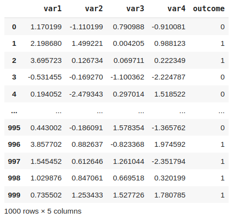
This data frame has 1000 rows, with four variables (3 informative) and one target (categorical binary outcome):

Based on this starting data, let’s introduce missing data following MCAR, MAR, and MNAR.

1. MCAR: Introduces missing values completely at random on variable 1:

df_mcar = df.copy()
mcar_mask = np.random.rand(len(df)) < 0.2 # random sample
df_mcar.loc[mcar_mask, 'var1'] = np.nan

1. MAR: Introduces missing values at random at var1 based on observed var2:

df_mar = df.copy()
mar_mask = df['var2'] > df['var2'].median()
df_mar.loc[mar_mask, 'var1'] = np.nan

1. Introduces MNAR: Introduces missing values not at random at variable 1:

df_mnar = df.copy()
mnar_mask = (
    ((df['var1'] > df['var1'].quantile(.8)) & (df['outcome'] == 1)) |
    ((df['var1'] < df['var1'].quantile(.4)) & (df['outcome'] == 0))
)
df_mnar.loc[mnar_mask, 'var1'] = np.nan

Finally, let’s combine them into a dictionary to facilitate usage later on:

missing_datasets = {
    "MCAR": df_mcar,
    "MAR": df_mar,
    "MNAR": df_mnar
}

Want more easy to follow Python recipes for missing data imputation? Check out our Python Feature Engineering Cookbook. The most exhaustive book on feature engineering.

Analyzing the missing data impact

Visualizing the distributions

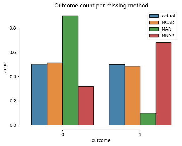
We will compare the proportion of the binary outcome for each dataset after applying the CCA technique (dropping all rows with missing data). This might give us some clue on how CCA changes the outcome distribution according to the missing pattern (MCAR, MAR, and MNAR).

The following code computes the proportion for each dataset, after applying CCA:

# Get outcome counts per missing pattern + actual counts
actual = df['outcome'].value_counts(normalize=True).to_frame('actual')
missing = [
    data.dropna()['outcome'].value_counts(normalize=True).to_frame(method)
    for method,data in missing_datasets.items()
]

Then, we can prepare the data for plotting and use it to plot the distributions:

# Prepare data for plotting with seaborn
data = (
    pd.concat([actual, *missing], axis=1)
    .reset_index()
    .melt(id_vars='outcome')
)

# Plot outcome counts per missing pattern + actual counts
sns.barplot(
    data=data,
    x='outcome', y='value', hue='variable',
    edgecolor='black',
    alpha=.9
)

plt.legend(loc='best')
plt.title('Outcome count per missing method')
sns.despine(trim=True, offset=10)
plt.show()

The resulting plot shows that the proportion for both binary outcomes is similar between the actual dataset and the missing one with MCAR, while we can see a notable difference for MAR and MNAR:

Let’s also create a function to visualize the distribution of the target variable according to variable 1 on the distinct missing patterns we’ve just introduced:

def plot_missing_values_by_outcome(df, var, title=None, ax=None):
    if not ax:
        fig, ax = plt.subplots()
    df_plot = df.assign(var_missing_flag = df[var].isna()).copy()
    sns.violinplot(data=df_plot, x='var_missing_flag', y='outcome', ax=ax, color='black')
    ax.set_title(title)
    ax.set_xlabel('Missing value flag')
    return ax

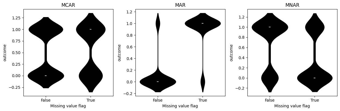
This function receives a dataframe, and compares the outcome distribution according to a target variable. Let’s set variable 1 as the target one since it’s the one we’ve introduced missing values using distinct missing patterns (aka MCAR, MAR, and MNAR).

Let’s apply this function to the missing datasets, creating side-by-side plots:

fig,axes = plt.subplots(ncols=3, figsize=(12,4))
for ax, missing_method in zip(axes, missing_datasets):
    plot_missing_values_by_outcome(
        missing_datasets[missing_method], 'var1',
        title=missing_method, ax=ax
    )

plt.tight_layout()
plt.show()

The resulting plot shows how that MAR and MNAR have distinct distributions for records with missing values:

Comparing model coefficients

We can use a regression model to assess how CCA distorts the coefficients in distinct scenarios. We can expect unbiased estimates for MCAR, while both MAR and MNAR can impact the regression analysis.

We’ll use the following function to compute the regression coefficients:

def get_cca_coefs(incomplete_data, dataset):
    """Apply CCA & return regression coefficients for regressions analysis"""
    # Apply CCA
    complete_cases = incomplete_data.dropna() # missing x is filled
    # Split features and target
    X_complete = complete_cases.drop(columns='outcome')
    y_complete = complete_cases['outcome']
    # Train the logistic regression algorithm
    model = LogisticRegression(random_state=42)
    model.fit(X_complete, y_complete)
    # Retrieve coeficients
    coefs = pd.Series(model.coef_[0], index=model.feature_names_in_, name=dataset)
    return coefs

First, we compute the coefficients for the complete data (our “ground truth”):

# Retrieve coefficients for complete data
X_full, y_full = df.drop(columns='outcome'), df['outcome']
model_full = LogisticRegression(random_state=42)
model_full.fit(X_full, y_full)

full_coefs = pd.Series(model_full.coef_[0], index=model_full.feature_names_in_, name='full')

Then, we can compute the coefficients for the incomplete data while combining into a single table:

df_coefs = pd.concat([
    full_coefs,
    get_cca_coefs(df_mcar, 'mcar'),
    get_cca_coefs(df_mar, 'mar'),
    get_cca_coefs(df_mnar, 'mnar')
], axis=1).T

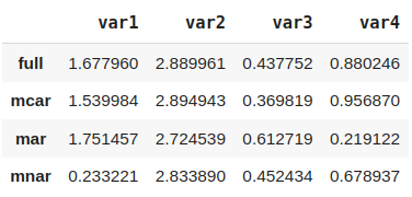
The output of df_coefs shows that mcar was the most similar to the full dataset, while mar and mnar have notable changes on var 1 or 4:

What else could we do to explore these relationships?

We can further extend this data analysis by including stats like standard errors, confidence intervals, etc. For instance, the Wald Test allows us to assess if two linear regression models’ coefficients are statistically different. The Little’s MCAR test (see references at the end of the blog) checks whether the pattern of “missingness” is independent of observed and unobserved data.

CCA Pipeline with Feature-engine

Let’s wrap up this coding section with a practical machine learning pipeline using Feature-engine’s DropMissingData transformer, which provides a convenient way to apply Complete Case Analysis within a scikit-learn pipeline.

This class automatically removes rows with missing values, ensuring that only complete cases are used for model training and evaluation. Below is an example of how to implement this in a pipeline:

from feature_engine.pipeline import Pipeline
from feature_engine.imputation import DropMissingData
from sklearn.model_selection import train_test_split

# Split MCAR dataset into training and test sets
X, y = df_mcar.drop('outcome', axis=1), df_mcar['outcome']
X_train, X_test, y_train, y_test = train_test_split(X, y, test_size=0.2, random_state=42)

# Create a ML pipeline with CCA strategy to handle missing values
model_pipeline = Pipeline(steps=[
    ('drop_missing', DropMissingData()),
    ('logistic_regression', LogisticRegression(random_state=42))
])

# Train model with pipeline
model_pipeline.fit(X_train, y_train)

Since we haven’t specified any variables in DropMissingData(), the transformer will drop all observations with missing values in any feature, effectively applying Complete Case Analysis (CCA). We can then use model_pipeline.predict(X_test) to generate predictions only for the observations with complete cases.

Build better feature engineering pipelines with Feature-engine and Scikit-learn with easy to follow tutorials in our course Feature Engineering for Machine Learning.

Let’s also inspect the number of observations for the training and test sets before and after applying the transformation, as well as the number of predictions:

print(f"""
Original training data size: {len(X_train)}
Transformed training data size: {model_pipeline[0].transform(X_train).shape[0]}
Predictions for the training data: {model_pipeline.predict(X_train).size}

Original test data size: {len(X_test)}
Transformed test data size: {model_pipeline[0].transform(X_test).shape[0]}
Predictions for the test data: {model_pipeline.predict(X_test).size}
""")

Below, we see the size of the training and testing set before and after applying CCA:

Original training data size: 800
Transformed training data size: 653
Predictions for the training data: 653

Original test data size: 200
Transformed test data size: 165
Predictions for the test data: 165

As a result, we observe fewer observations in the transformed data for both the training and test sets due to the removal of incomplete cases. The number of predictions matches the size of the transformed datasets, confirming that the model only generates predictions for complete cases.

Alternatives to CCA

While Complete Case Analysis (CCA) is simple and easy to implement, it is not always the best approach, especially when dealing with MAR or MNAR mechanisms or when a significant portion of the data is missing. Below are some common alternatives to CCA, including distinct imputation models available in libraries like scikit-learn and Feature-engine.

1. Simple Imputation

• Mean/Median/Mode: Replace missing values with column statistics. The imputed values take the mean, median or mode of the variable being imputed.

• Constant Value: Replace with predetermined, i.e., arbitrary values.

2. Advanced Imputation

• KNN imputation: Imputes based on similar observations
• MICE: Multiple imputations through predictive models

3. Missing Indicators

• Add binary features showing “missingness”

All these methods (and more!) are freely available on scikit-learn and Feature-engine.

Conclusions

Complete Case Analysis (CCA) is a straightforward and efficient method for handling missing data, particularly when the “missingness” is MCAR and the proportion of missing values is small. However, its limitations become apparent when dealing with MAR or MNAR mechanisms or when a significant portion of the data is missing. In such cases, CCA can introduce bias, reduce statistical power, and distort the underlying relationships in the data.

To address these limitations, missing data imputation methods offer more robust solutions. Techniques like simple statistical imputation, constant values, KNN imputation, and MICE can help preserve data integrity and improve the validity of your analyses. Libraries like scikit-learn and Feature-engine provide powerful tools to implement these methods efficiently.

Ultimately, the choice of method depends on the missing data mechanism, the amount of missing data, and the specific requirements of your analysis. By carefully assessing the nature of missingness and selecting the appropriate handling strategy, you can ensure more accurate and reliable results in your machine learning and statistical analyses.

References

• Scikit-learn Documentation: Imputation
• Feature-engine Documentation: Imputation
• Rubin, D. B. (1976). Inference and Missing Data. Biometrika.
• Little, R. J. A. (1988). A Test of Missing Completely at Random for Multivariate Data with Missing Values. Journal of the American Statistical Association.
• Knol, M. J. et al. (2010). Unpredictable bias when using the missing indicator method or complete case analysis for missing confounder values: an empirical example. Journal of Clinical Epidemiology.

Additional resources

Check out our course Feature Engineering for Machine Learning to learn more about these and other ways to handle missing values, focusing on preprocessing data for machine learning.