
Is Boruta dead?
Boruta is a feature selection algorithm described in 2010 by a group of bioinformaticians to select features in biological systems, where we normally work with thousands of variables (e.g., gene expression).
If I am honest, back then, I had a quick look at the logic of the Boruta algorithm, thought it was an over-complicated extension of the importance derived from random forests, and left it there without paying further attention.
Since then, the buzz about Boruta on social media and data science competition websites like Kaggle dissipated, so I wondered if the method was finally dead.
It turns out, it is not.
Boruta is not dead
As of March 2025, the term “boruta” is searched about 8 thousand times per month on google around the world. Similarly, the Python library “boruta” is downloaded an astonishing 230 thousand times per month.
Judging by these numbers, the boruta feature selection algorithm is further from dead. Hence, I decided to finally have a look at the ins and outs of Boruta, and gather my thoughts around this feature selection model.
If you’re looking to dive deeper into practical feature selection techniques (including Boruta), check out my book on Feature Selection for Machine Learning.
Here we go.
Boruta, what is it?
The idea behind Boruta is simple: we make a randomized copy of the dataset, add the copy to the original variables and train the classifier for this extended dataset. To assess variable importance, we compare the importance of the original variables with that of the randomized variables. If it is greater, we keep the features. If not, bye bye.
In Boruta, the classifier is a random forests and the randomized copy of the variables are called shadow features or shadow attributes. Keep these terms in mind for the coming paragraphs.
Boruta algorithm
On high level, Boruta works as follows:
- Train several random forests using the variables and their randomized versions.
- Derive feature importance.
- Determine if each feature’s importance is greater than the maximum importance shown by the shadow features.
- If a feature’s importance is greater than the max of the shadow attributes a significant number of times (remember that we trained several random forests), then that feature is selected.
Now some details:
Each random forest training process in step 1 is called an iteration.
The significance in step 4 is tested by a two-tailed binomial distribution test. In short, if we train 10 random forests, and the feature is important, we expect its importance to be greater than the shadow features more than 5 times. This can be statistically determined by the binomial distribution.
Boruta algorithm in detail
Looking at the source code of Boruta, this is the detailed implementation:
- Create a randomized copy of the dataset (shadow features) and add it to the original data.
- Train a random forest model.
- Obtain feature importance for original and shadow features.
- Make a statistical test to identify features whose importance is significantly greater than that of the maximum of the shadow attributes.
- Select the features in 4.
- Repeat steps 1-5 with the remaining features.
Statistical testing of features
On step 4, one of three things can happen:
- A feature is statistically more important than the shadow attributes, and then it is selected.
- A feature is statistically not different from the shadow attributes, and then it is removed.
- It is unclear if a feature is statistically different or not (i,e., we need more iterations).
At the end of each iteration (steps 1-5), features in 1 are selected, features in 2 are removed, and features in 3 are called “tentative” and passed to the next round.
Want to go beyond the theory and see Boruta (and other feature selection methods) in action? Check out my course on Feature Selection for Machine Learning, where we cover practical implementations with Python and real datasets.
Number of iterations
How many times should we repeat the procedure? Well, this is somewhat unclear. As users, we need to provide an arbitrary number of repetitions for step 6.
The authors of Boruta suggest 12 as a starting point. If at the end of 12 iterations we still have a lot of tentative features, we should increase the number of iterations.
Obviously, the more iterations the more confidence we have when selecting or rejecting features. The trade-off is, as always, computation time.
Something that leaves me scratching my head
What I don’t completely understand, is why we run a binomial test after each iteration, instead of training all the iterations of random forests first, and then carrying out the test once.
Obviously, when n is larger (and by n, I mean the number of iterations or the number of random forests, which results in the number of times a feature was deemed more important than the shadow features), we’ll have more confidence in the result of the binomial distribution test (a consequence of the sample size effect).
In simple words, if a feature was more important than the shadow attributes 1 out of 1 iteration, provides less information than when a feature was more important than the shadow attributes 1 out of 10 iterations. That is true for us and also for the binomial distribution test.
In short, with more iterations, more confidence on the selection process.
Instead, the authors decided to examine each feature’s importance at every round. So the first selections or rejections will have less confidence than the later ones, when n is larger.
My guess is that this decision was made to make the Boruta algorithm run faster. If we manage to reduce the number of features early on, later iterations which are trained on the remaining (i.e., tentative) features will take less time to compute.
But this comes with its drawbacks: over multiple iterations, we are testing the same feature over and over, so we increase the false discovery rate (more on this later).
Python and R implementation of Boruta
There are 2 popular open-source Boruta implementations, one in R created by the authors of Boruta, and one in Python adapted from that in R.
How do these implementations differ?
The Python library was based on the R library, but later on made some modifications that provide more flexibility during the selection process. Here is how they differ:
Feature importance
Feature importance is derived differently in the R and Python implementation.
In R, we use the decrease in accuracy obtained by feature permutation, which is called by the authors the z-score.
In Python, we use the importance derived from the random forest itself, which consists in the decrease in impurity returned by a feature across all trees in the forest.
Threshold to deem a feature important
In R, we flag a feature as important if its importance is greater than the maximum importance of any of the shadow attributes.
In Python, we can be more flexible and use a smaller threshold, like a percentile instead of the maximum. Like this, we can control if we want to be more or less conservative during the selection procedure.
Model to determine feature importance
In R, we use random forests for the selection procedure. In Python, we can use any tree based model, like gradient boosting machines and related models like lightGBMs and XGBoost.
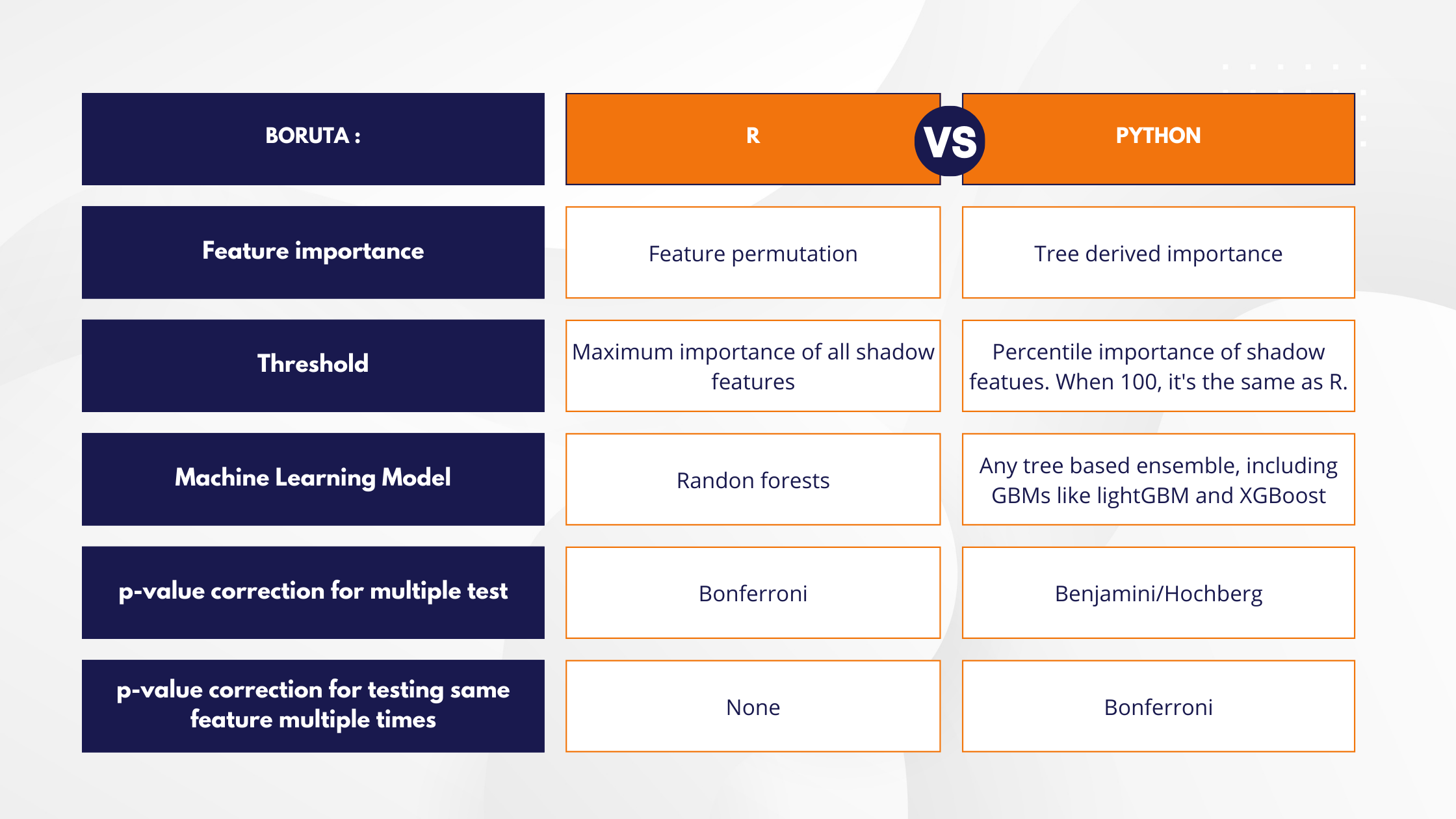
P-value correction
To determine if a feature’s importance is significantly greater than the shadow attribute, we compare it’s importance to the maximum (or percentile) importance of all shadow features with a binomial distribution test.
The binomial distribution test relies on:
- The number of times (here iterations) in which the feature’s importance was greater than the shadow,
- the total number of iterations ran so far, and
- the binomial random probability which is 0.5 in this case.
Because we are testing thousands of features, we are making thousands of binomial tests. Hence, we need to correct the p-value for multiple testing.
In R, we use the Bonferroni correction. In Python we use the less conservative Benjamini/Hochberg p-value correction for false discovery rate.
Same feature tested multiple times
In addition, tentative features are tested over several iterations. In short, we test the tentative features over and over.
To address this issue, the Python implementation uses a Bonferroni correction over the number of iterations. The R implementation does not deal with this issue.
Master feature selection in Python with my course on Feature Selection for Machine Learning, the most exhaustive course on feature selection available online.
What is Boruta trying to address?
According to the authors, in large datasets spurious correlations among variables are common.
The feature importance derived from decision trees and random forests is affected by correlation. In general, correlations return lower feature importance values. So, in principle, variables with spurious correlations may show decreased importance compared to other, less important variables, that randomly happened not to be correlated with other features. A bit of a stretch if you ask me.
By introducing randomized features, we should, in theory be also creating random correlations, which will be captured in the importance of the shadow variables, and that would help us address truly important features, even if, they are randomly correlated with other variables.
In addition, a simple value of importance doesn’t provide a statistically valid measure to select or reject a variable. Hence, the introduction of the binomial distribution tests.
What about correlations that are not spurious?
That is, unfortunately, not taken care of by Boruta.
We know that variables that are correlated will show decreased importance derived from random forests.
But here is the thing: Boruta is not trying to rank variables by importance. Its aim is to select features that are significantly associated with the target, regardless of their ranking. So in this sense, Boruta succeeds. As a ranking algorithm, not so much, but it was never its intention.
Is it worth the fuss?
At first sight, Boruta looks complicated. We train several random forests, we introduce random variables and then we compare the importance values with a statistical test. In fact, training several rounds of random forests increases computation time quite substantially. So, is it worth it?
For statistical purposes, I am inclined to say yes. When we do research, we rely on statistical methods that assign a degree of significance to a value or a series of values, so that we can accept or reject hypothesis (here, features) with confidence, and understand the error that we make when accepting or rejecting those hypothesis.
In fact, we do need p-values to write scientific conclusions in scientific articles.
This is why Boruta uses statistical tests and corrects the p-values to reduce the false discovery rate. Boruta was designed within a scientific environment for scientific purposes, so these are required requisites.
And in machine learning?
In Machine learning, we are usually interested in making simpler, faster and robust models. That’s the main reason we do feature selection.
We are not generally interested the statistical relevance of every feature, we often make compromises and accept smaller or different subset of features that result in good enough machine learning model performance.
So in machine learning, Boruta provides an additional tool to select features, but I would not call it the one-stop-solution for all relevant feature selection. Far from that.
The main criticism that I would make to Boruta is that it is slow: training multiple random forests takes time. And to assess thousands of features we need random forests with numerous trees to ensure that all features are included in a tree at least once. That increases computation time even further.
In addition, as I discussed in a previous paragraph, Boruta does not address the decreased importance due to variable correlations, so the rankings we derive from it are not super meaningful.
But fortunately, in machine learning, there are other feature selection methods that we can use.
Boruta with Python – demo
Now that I’ve finished gathering and discussing my thoughts about Boruta, let me wrap up with a Python demo on how to use Boruta.
I’ll use the Madalon dataset, which is an artificial dataset used in NIPS2003. This dataset contains 2000 observations and 500 features.
Let’s begin by importing the libraries and functions that we need for the demo, including Python‘s boruta package:
import matplotlib.pyplot as plt
import pandas as pd
from sklearn.ensemble import RandomForestClassifier
from boruta import BorutaPy
Let’s make a function to load the data:
def load_data():
    # URLS for dataset via UCI
    train_data_url='https://archive.ics.uci.edu/ml/machine-learning-databases/madelon/MADELON/madelon_train.data'
    train_label_url='https://archive.ics.uci.edu/ml/machine-learning-databases/madelon/MADELON/madelon_train.labels'

    X_data = pd.read_csv(train_data_url, sep=" ", header=None)
    y_data = pd.read_csv(train_label_url, sep=" ", header=None)
    data = X_data.loc[:, :499]
    data['target'] = y_data[0]
    return data
Now, let’s load the data into a dataframe:
data = load_data()
Let’s display the first 5 rows:
data.head()
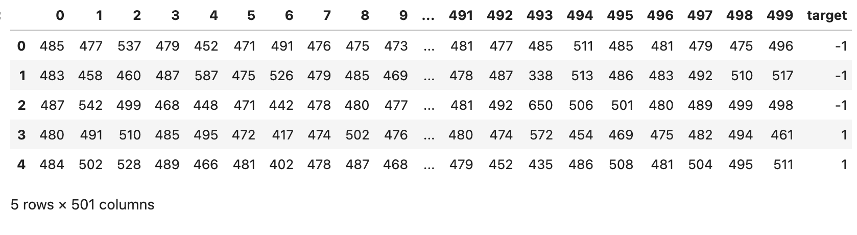
In the following image, we see the first 5 rows of the Madalon dataset:
Now, we split the data into predictors and target variable:
y = data.pop('target')
X = data.copy().values
Let’s now set up the random forest classifier that we’ll use for the feature selection:
rf = RandomForestClassifier(
n_jobs=-1,
class_weight=None,
max_depth=3,
random_state=0,
)
Note, that I do not set the number of trees for the forest. That’s because the Python implementation can find an optimal number of trees that maximizes the probability of examining every feature in the dataset at least once.
The more features, the more trees we need in the ensemble.
Now, we set up the Boruta feature selection process:
feat_selector = BorutaPy(
estimator = rf,
n_estimators='auto',
perc=100,
alpha=0.05,
two_step=True,
max_iter=20,
verbose=2,
random_state=0,
)
There are a number of important parameters in this implementation:
- estimator is the machine learning model to use in the selection. It can be random forests or other tree based model.
- n_estimators is the number of models in the ensemble. With auto, the Python implementation decides the best number of trees to evaluate all features in the dataset. Alternatively, we can set it to a specific integer. Remember that more features will require more trees in the ensemble for a fair assessment.
- perc: if 100, then a feature is deemed important if its importance is greater than the maximum importance of the shadow features. If we set it to 90, then, a feature will be deemed important if it is greater than the 90th percentile of the shadow features. The lower the percentage, the more conservative the selection (i.e., we select more features).
- alpha is the value of hypothesis rejection. In general, we use 0.05, but you can change it. Higher values are more conservative.
- two_step: This is a less intuitive parameter. If False, then the implementation will carry out Bonferroni for p-value correction given that we are testing multiple features. If True, it will use the Benjamini/Hochberg correction for the multi-feature comparison, AND also the Bonferroni correction to accommodate the fact that the same feature is tested over and over along the multiple iterations.
- max_iter is the number of times to train the random forests. More times mean better assessment of the features AND also higher computation cost.
- verbose is used to print out (or not) intermediate steps during the process of the algorithm.
- random_state, well, it goes without saying. We are adding random variables and using random forests, so this parameter is a must.
Now, we trigger the feature selection process:
feat_selector.fit(X, y)
Since we set verbose to 2, we’ll see displayed intermediate steps of the selection process. I will only print out the results of the 8th iteration:
Iteration: 	8 / 20
Confirmed: 	0
Tentative: 	22
Rejected: 	478
We see that after training 8 random forests, we reject 478 features as not-significantly different from the shadow attributes, we selected 0 so far, and we remain to evaluate 22 features.
After the selection process is done, we can print out the number of selected features like this:
print ("Selected Feature Matrix Shape")
print (feat_selector.support_.sum())
We’ve selected 17 features from the original 500:
Selected Feature Matrix Shape
17
The Python boruta implementation offers a feature ranking, which we can capture in a series like this:
ranking = pd.Series(feat_selector.ranking_, index=data.columns)
- Selected features show ranking 1 and can be identified like this: ranking[ranking ==1]
- Unclear or tentative features show ranking 2, and can be identified like this: ranking[ranking ==2]
- The features that were removed show higher rankings.
Let’s plot the rankings of the removed features:
ranking[ranking > 2].sort_values().head(20).plot.bar()
plt.ylabel("ranking")
plt.xlabel("feature")
plt.title("ranking of non-selected features")
plt.show()
In the following visualization, we see the rankings of the features that weren’t selected:
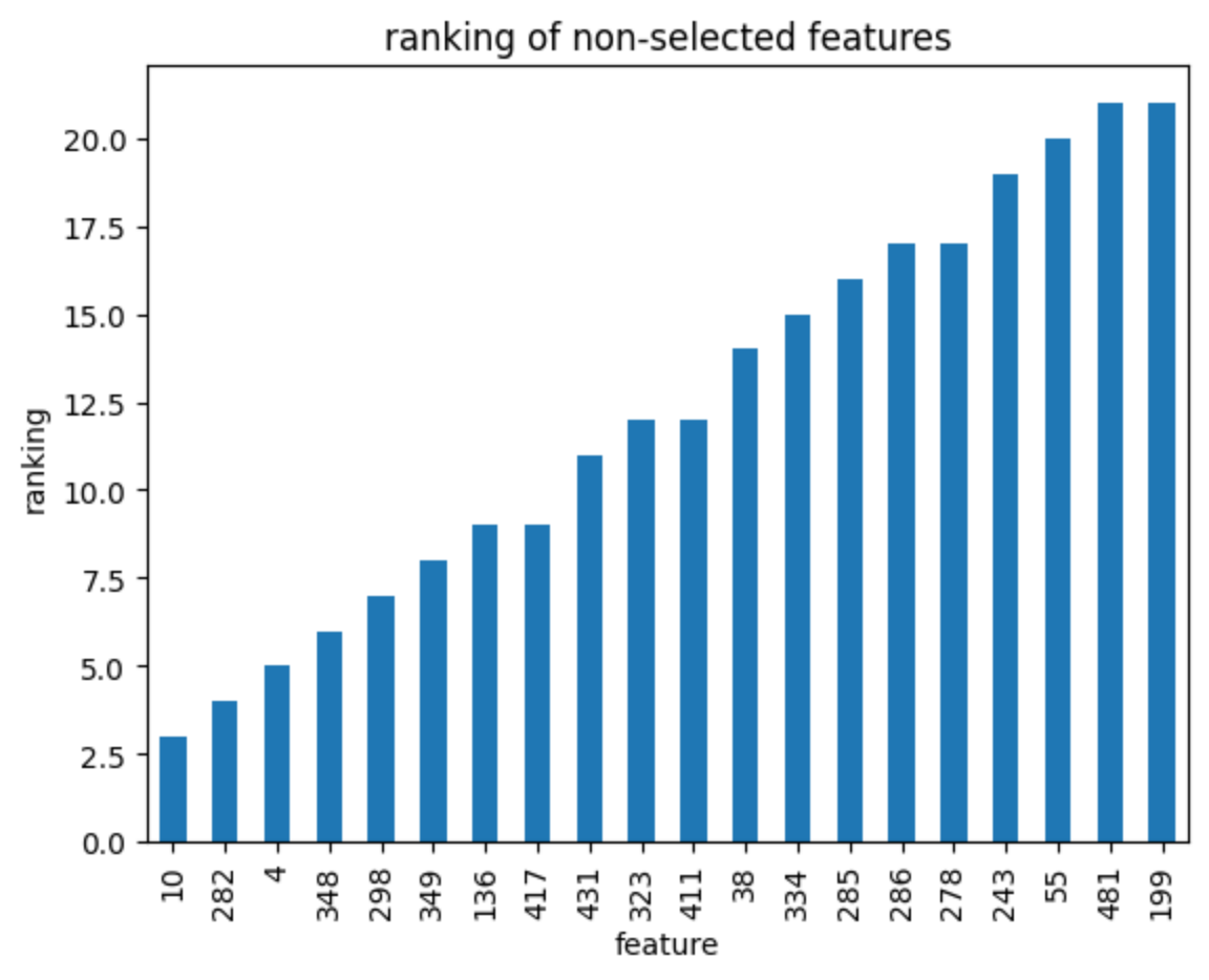
As discussed previously, I don’t think that the aim of Boruta was to rank features, so please take this rankings with a grain of salt.
Finally, to reduce the dataset to the selected features:
X_t = feat_selector.transform(X)
And now, if we check how many features remain in the transformed dataset, we should see 17:
X_t.shape
And that is indeed, what we see:
(2000, 17)
And that’s it! I finished rambling about Boruta.
References
You can find more about Boruta in:
👉 The original article
👉 The R library article
You can implement it on Python with BorutaPy
To learn more about feature selection, enroll in my course Feature Selection for Machine Learning.

Or if you prefer reading, my book Feature Selection in Machine Learning:

See ya!
