Imbalanced Data in Machine Learning: Techniques and Best Practices

Imbalanced datasets are a familiar challenge data scientists and machine learning practitioners face. When the distribution of classes in a dataset is skewed, one or more classes have significantly fewer samples than others.

But does that mean we need to balance the data before training a model? In most tabular classification projects, that should not be our starting point.

Much of the advice about handling imbalanced data gets this wrong. It presents undersampling, oversampling, SMOTE, or class weights as necessary fixes for an unequal class distribution. This leads people to spend time resolving an imbalance that simply reflects the real world, without checking whether it is causing a problem at all.

My starting recommendation is to train a strong classifier on the original data, tune it using log loss or the Brier score, and evaluate its probability predictions. If we need class labels, we can then adjust the classification threshold to reflect the decisions we want to make.

This article will explore the following:

• The nature of imbalanced data
• The challenges of imbalanced datasets
• What undersampling, oversampling, and SMOTE actually do
• Cost-sensitive learning
• How to evaluate probabilities and make cost-sensitive decisions, and
• Ensemble models for imbalanced datasets

We will also look at imbalanced-learn, an open-source Python package for experimenting with resampling methods.

For a video introduction to these ideas, check out:

For the reasoning behind these recommendations and practical Python examples, check out my recent book Imbalanced Data: Myths, Mistakes and Modern Solutions.

What is Imbalanced Data?

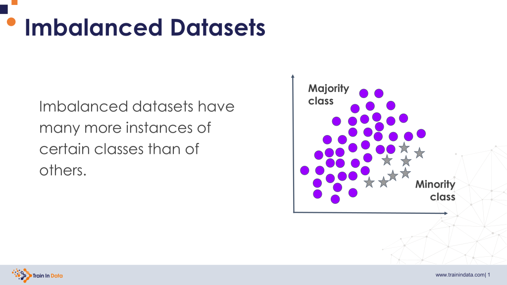
In imbalanced datasets, one class is significantly more represented than the other(s).

Imbalanced datasets are common in the real world. Fraudulent purchases, rare diseases, and customer churn can all occur less often than their alternatives. A balanced dataset has roughly similar numbers of observations in each class, but equal counts are not a general requirement for machine learning.

The degree of imbalance can vary significantly and may be caused by a naturally unequal distribution or sampling bias in data collection. These are different situations. A dataset that reflects a rare event accurately does not need correcting simply because that event is rare.

Binary vs. Multiclass Imbalanced Data

Binary imbalanced data refers to datasets with only two classes: one class has a majority of samples and the other a minority.

In binary classification tasks, imbalanced datasets occur when one class has significantly fewer samples than another (e.g., 80% of samples belong to Class A while only 20% belong to Class B). This phenomenon is also known as “class imbalance.”

On the other hand, multiclass classification involves three or more classes, where one or more classes may have significantly fewer samples than others.

A real-life example of a multiclass imbalanced dataset is a medical diagnosis dataset. There will be multiple diseases or different classes; one may have a lower occurrence rate than others.

One question I hear far too often is: “When should we consider a data set imbalanced?” The answer is straightforward: if you have different proportions of each class, it is an imbalanced data set. That doesn’t mean, however, that you automatically need to reach out for resampling, class weights or SMOTE. Read on.

Minority Class vs. Majority Class

In both binary and multiclass imbalanced data, we’ll find:

• Minority classes: These are the classes with fewer samples than others. They are often associated with rare events.
• Majority classes: These are the most frequent classes in a dataset, having more samples than other classes.

Why is Imbalanced Data Challenging for Machine Learning?

Often, problems attributed to class imbalance stem from completely different reasons, which are: insufficient data, poor class separability or using the wrong machine learning model or evaluation metrics. Let’s look at them in more detail.

Too Few Minority-Class Examples

Model performance typically improves with more data, but only up to a point. With imbalanced datasets, what matters is not just the proportion of minority observations but their absolute number: a thousand positives in a million rows carry more information than ten positives in a thousand, even though both are a 1% positive rate.

Learning curves, which plot training and validation performance as the dataset grows, show whether more data would still help or whether performance has already plateaued.

Poor Class Separability

How well a model separates the classes depends on whether the available features actually distinguish them, not on how many examples of each class we have. A model trained on a thousand apples and a single orange will still classify the orange correctly if colour alone tells them apart; separating an orange from a clementine is much harder.

Separability can be assessed directly: an ROC-AUC close to 1 indicates the classes are highly separable, while a value near 0.5 indicates substantial overlap. When separability is poor, balancing the class counts will not supply the missing information, better features will.

Choosing the Wrong Model

Model choice affects imbalanced classification more than the imbalance ratio itself. Simpler models, like logistic regression or a single decision tree, struggle when the minority class follows a complex, non-linear pattern, while more flexible models, like random forests and gradient boosting machines, can often separate the classes effectively.

Misleading Evaluation Metrics

Accuracy is the clearest offender: on a dataset with 99 majority observations per minority one, always predicting the majority class scores 99% accuracy while catching no minority cases at all.

Precision, recall, or F1 are alternatives that allow us to understand if a model discriminates among the classes. However, many practitioners use them wrongly, by not adjusting the decision threshold used to calculate their values.

All these metrics are threshold dependent: changing the threshold used to assign a sample to a class changes their values, so we need to adjust it too. The default of 0.5 will lead us into wrong conclusions.

Undersampling, Oversampling and SMOTE

If we have few observations of the class we care about most, why not add more, or remove some from the majority, to give it more visibility? This is the logic behind resampling methods, and it is sound.

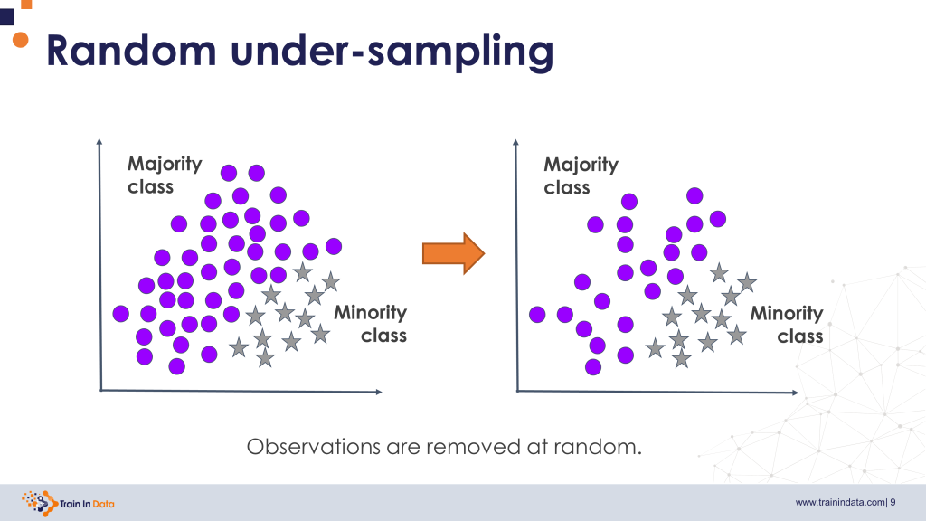
Undersampling removes observations from the majority class until the two classes reach a chosen ratio. Random undersampling does this by discarding majority observations at random, while cleaning methods like Tomek links or edited nearest neighbours target observations sitting close to the decision boundary instead.

Oversampling adds observations to the minority class instead. Random oversampling duplicates existing minority rows, while SMOTE generates new ones by interpolating between a minority observation and its nearest minority neighbours, producing synthetic points that sit between real ones.

Giving the minority class more weight, duplicating its observations, or removing majority class observations changes the relative influence of the classes during training, which can raise recall at the cost of more false positives, without necessarily showing that the model discriminates the classes any better.

We can often obtain that same change in decisions by training on the original data and lowering the threshold afterward.

Resampling, Class Weights and Threshold Tuning Are Equivalent

Resampling, class weights and threshold tuning are equivalent ways of making cost-sensitive decisions: rather than changing the training data itself, they change how much each type of error counts.

A cost-sensitive decision incorporates the cost at the time of making a decision. For example, rejecting a high value credit card transaction might be the correct cost-sensitive decision, even if the probability of the transaction being fraudulent is low: we incorporate the cost of disbursing the money to the fraudster into the decision.

Cost-Sensitive Learning

Let’s continue with our fraud detection example: a fraudulent transaction is the positive class (1), a legitimate one the negative class (0), and we can either approve or reject a transaction.

Suppose missing fraud costs us 9 units and rejecting a legitimate transaction costs 1 unit, with no cost for correct decisions. We can put these costs into a cost matrix, with our decisions in the rows and the actual outcomes in the columns:

Our decision	Actually legitimate (0)	Actually fraudulent (1)
Approve the transaction (predict 0)	0	9, false negative
Reject the transaction (predict 1)	1, false positive	0

Now consider a transaction with a 20% chance of being fraudulent. Approving it carries an expected cost of 0.2 * 9 = 1.8, while rejecting it carries 0.8 * 1 = 0.8. Rejecting has the lower expected cost, so we would reject it, even though fraud is the less likely outcome.

Making Cost-Sensitive Decisions

Let’s call the probability of fraud p, and the weights w1 (fraudulent, 9) and w0 (legitimate, 1). Many data scientists bring these costs into training through class weights, which multiply each class’s contribution to the loss function they use to fit the model.

Weighting changes the quantity the model effectively targets. Starting from p = 0.2, multiplying by the weights gives 1.8 for fraud and 0.8 for legitimate; dividing 1.8 by their sum gives an adjusted probability q of about 0.69:

q = w1 * p / (w1 * p + w0 * (1 - p))

Since q exceeds 0.5, the weighted model rejects the transaction at the default threshold. The actual probability of fraud is still 20%; the weights have simply changed what the model learns to predict.

Threshold Tuning

We can reach the same decision by adjusting the threshold on the original probability instead. The two actions have equal expected cost when 9 * p = 1 * (1 - p), at p = 0.1; above that, rejecting the transaction is cheaper. More generally, that cutoff is w0 / (w0 + w1), the false-positive cost divided by the sum of both error costs, and applying it to p gives the same decisions as applying 0.5 to q. Our transaction’s probability of 0.2 exceeds 0.1, so we reject it either way.

Resampling is Equivalent to Threshold Shifting

The relationship between resampling (oversampling or undersampling) and cost-sensitive decisions has a long theoretical history; see Elkan’s foundational paper.

In short, oversampling to increase the number of minority class examples, or undersampling to reduce the number of majority class examples, is achieving the same thing as class weighting: it moves the decision boundary the model learns, so that at the default threshold of 0.5, we can still make cost-sensitive decisions.

Where the Advice to use SMOTE or Rebalance the Data Came From

Random forests and the first gradient boosting machines were introduced in 2001. The stronger, modern implementations, XGBoost, LightGBM, and CatBoost, arrived later still: 2016, 2017, and 2019.

Most undersampling methods predate 2001 altogether, so they were evaluated with the classifiers available at the time: nearest-neighbour models and decision trees. The original SMOTE paper followed in 2002, just after random forests and gradient boosting were published, and its evaluation focused on decision trees and Naive Bayes.

The SMOTE variants published since then keep testing on similarly simple classifiers: decision trees, SVMs, logistic regression, and k-nearest neighbours. Much of the evidence behind familiar resampling advice still comes from that earlier generation of models, evidence that says little about whether the same preprocessing helps a modern boosted model.

To SMOTE or Not To SMOTE

A 2022 comparative study evaluated a range of classifiers, including decision trees, support vector machines, and multi-layer perceptrons, across multiple imbalanced datasets. SMOTE improved these models, which also turned out to be the ones most sensitive to class imbalance in the first place.

The same study found that XGBoost and CatBoost separated the classes effectively on their own, and applying SMOTE offered no additional benefit.

In my recent book, Imbalanced Data: Myths, Mistakes and Modern Solutions, I show that class weights and undersampling shift the decision boundary rather than genuinely improving model performance. I also cover the historical context these methods were developed in, test whether the evidence supports using them with stronger classifiers, and offer best practices for working with imbalanced datasets.

How to Handle Classification Problems in Imbalanced Data

My recommendation for tabular data is to establish a strong baseline on the original class distribution, evaluate its probabilities, and then choose how to turn those probabilities into actions.

Choosing Correct Evaluation Metrics

Accuracy alone can hide poor performance on the class we care about, as we saw earlier with the 99% accuracy trap. Replacing it with F1 score while keeping the default threshold does not solve the evaluation problem either. We need to distinguish three types of assessment:

What we want to assess	Evaluation metrics	Threshold dependent
Quality of probability predictions	Log loss, Brier score	No
Ranking of observations	ROC-AUC, average precision or PR-AUC	No
Decisions made from predictions	Precision, recall, F1 score, balanced accuracy, MCC	Yes

For model selection and hyperparameter tuning, my preferred starting point is log loss or the Brier score. These are strictly proper scoring rules: their best value is achieved by predicting the true conditional probabilities. Log loss penalizes confident errors heavily; the Brier score measures squared differences between probabilities and outcomes.

ROC-AUC assesses how well positive observations rank above negative ones. A precision-recall curve helps us inspect the tradeoff between identifying positives and making false alarms; average precision and PR-AUC summarize that curve.

Ranking metrics do not establish probability calibration. A model can rank observations correctly while systematically overstating their risks.

Once a threshold is chosen, inspect precision, recall, and the confusion matrix, including true positives, true negatives, false positives, and false negatives. They complement probability evaluation. Keep in mind, however, that different metrics have different optimal thresholds: change the threshold, and the metric value changes too.

Train a Strong Classifier and Check Calibration

For tabular classification, start with a well-tuned model such as XGBoost, LightGBM, or CatBoost. Include a simpler baseline, such as logistic regression, when appropriate. Select hyperparameters using validation log loss or Brier score on data with the target population’s class distribution.

Do not automatically enable class balancing just because a library provides the option. XGBoost’s own parameter-tuning guidance distinguishes ranking performance from estimating probabilities and advises against rebalancing for the latter.

A calibrated model should assign probabilities that match observed frequencies: among cases assigned approximately 20% probability, roughly 20% should be positive. Proper scoring rules encourage accurate probabilities, but optimizing them does not guarantee calibration, so a lower Brier score alone does not prove it; check reliability diagrams too.

If necessary, assess calibration methods such as sigmoid (also known as Platt scaling) or isotonic scaling on held-out predictions, then evaluate the calibrated model on separate data. You can find Python examples in our article on probability calibration.

Using Cross-Validation

Cross-validation trains the model on different subsets of data, evaluates it on held-out subsets, and shows how much results vary across splits.

For independent observations, stratified cross-validation helps preserve class proportions. Check that each evaluation fold contains enough minority examples to support meaningful conclusions.

Keep a final test set untouched while selecting the model, calibration method, and threshold. Cross-validation does not rescue an unsuitable metric or data leakage.

Adding More Data

One practical way to improve generalization is to collect more representative observations, particularly with very few minority examples, and to check labels and improve the features that distinguish the classes.

Collecting genuine new examples is different from duplicating existing rows. Data augmentation, such as suitable image transformations, can encode useful domain knowledge, but its value needs testing. It is not evidence that arbitrary synthetic samples will improve a tabular classifier.

Adjusting the Threshold

Adjusting the classification threshold changes which observations receive a positive label. It does not improve the model’s underlying probabilities or ranking.

Choose the threshold on validation data or out-of-fold predictions to suit the application: expected cost, F1 score, or recall subject to an acceptable false-positive burden. Maximizing recall alone would allow the useless solution of flagging everyone.

ROC and precision-recall curves help us inspect candidate operating points. Scikit-learn provides TunedThresholdClassifierCV for this task, with a scoring function chosen for the application.

Training Set Resampling

Resampling changes the distribution of the training set through oversampling or undersampling; treat it as an experiment after establishing the baseline above, not a default step.

If you test it, split the data first and resample only inside each training fold, keeping validation and test distributions representative of deployment. Resampling before splitting lets duplicates or synthetic observations leak across the split, inflating performance, as the imbalanced-learn documentation demonstrates.

If a sampler or weighted model improves on that baseline in a fair comparison, we have a reason to use it. A higher recall at 0.5, on its own, is not that reason.

Overview of Undersampling

Random undersampling removes observations from the majority class at random. Cleaning variants like Tomek links and edited nearest neighbors remove observations near the decision boundary instead.

Pros

• Random undersampling can reduce storage requirements and model training time on very large datasets.

Cons

• Removing observations can discard useful information.
• Changing class proportions will distort estimated probabilities.

Overview of Oversampling

Random oversampling duplicates observations from the minority class at random and with replacement. SMOTE creates new data points by interpolating between observations. SMOTE was designed for continuous features. SMOTENC and SMOTEN extend it to mixed or purely categorical data, and ADASYN focuses new samples on regions where classes overlap most.

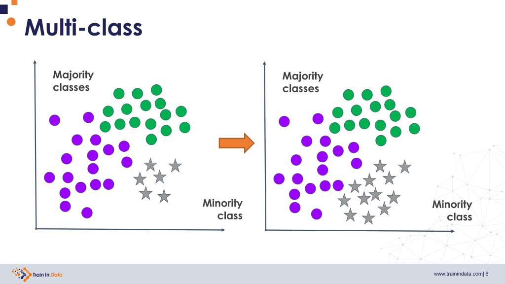
These methods add assumptions about what plausible new observations look like. An interpolated point is not a newly observed case, and it may fall in an overlapping region or represent an unrealistic combination of features.

I can’t think of a single pro of oversampling, so I will only say that this method should be considered when the dataset is small and gathering more data is not an option. For everything else, steer away from it.

Undersampling Or Oversampling: Which One to Choose?

Before choosing between them, establish whether either is needed.

If training time or memory is the constraint, random undersampling may offer a useful tradeoff. If predictive performance is the constraint, start by improving the model and its inputs instead: oversampling is not a replacement for collecting more information about the minority class.

“The classes are unequal” is not enough reason to choose either method.

Ensemble Models for Imbalanced Data

Ensemble models combine the predictions of multiple models, classical examples being random forests and gradient-boosting machines. They do not require balanced classes, so for this article’s tabular setting, XGBoost, LightGBM, and CatBoost are sensible candidates before introducing specialized sampling ensembles.

Examples of Ensemble Models for Imbalanced Data

Some ensemble methods incorporate resampling directly:

• Balanced Bagging: Resamples the training subsets used to fit the individual estimators.
• RUSBoost: Introduces random undersampling during boosting.
• EasyEnsemble: Combines AdaBoost learners trained on balanced samples.

These approaches have implementations in imbalanced-learn.

My advice: DO NOT use them.

For starters, they don’t outperform ensembles trained on the original data in their capacity to discriminate among classes. They also distort the calibration of the model’s probabilities.

Imbalanced-learn: The Open-Source Python Package for Working with Imbalanced Data

Imbalanced-learn, imported as imblearn, provides tools for experimenting with resampling and sampling-based ensembles: everything covered above, plus variants like cluster centroids, NearMiss, condensed nearest neighbor, and one-sided selection.

Samplers use a scikit-learn-compatible fit_resample(X, y), and an imbalanced-learn pipeline can apply resampling inside the training folds during cross-validation.

The library is useful when we have a reason to test these methods. Installing it and balancing every dataset should not be a routine preprocessing step.

Wrap-Up

Dealing with imbalanced data requires us to understand the prediction task, the available information, and the decisions we want to make. Unequal class counts do not establish that a dataset is broken.

Train a strong baseline on the original data. Tune probability predictions using log loss or the Brier score, inspect calibration, and use ranking metrics where appropriate. When you need class labels, select a threshold that reflects the application and evaluate the resulting decisions on untouched test data.

Undersampling, oversampling, SMOTE, and class weights should earn their place through a fair comparison. We should not add them simply because a tutorial says that imbalanced datasets need balancing.

For practical Python examples and a deeper discussion of the assumptions behind these methods, check out my book Imbalanced Data: Myths, Mistakes and Modern Solutions.