SMOTE in Python and whether you should still use it in 2025

In many real-world scenarios, data is imbalanced, meaning that one class (usually called the majority class) has many more samples than the other one (the minority class). Although you will read a lot that class imbalance makes it difficult for algorithms to classify the classes correctly, that is not necessarily the case. In fact, if the classes are well separated, that is, there is a clear separation boundary among them, the algorithms will work just fine. But when the class separability is not that clear, then things start getting difficult.

Read our “7 takes on working with Imbalanced Data“, were we discuss 3 recent articles that change the conversation about resampling and SMOTE. It’s free.

A quick note before we start: SMOTE does not make a model better at discriminating between classes. What it does is shift the model’s decision boundary so that, at the default classification threshold of 0.5, we make more cost-sensitive decisions — that is, we correctly flag a larger proportion of the minority class, which is usually the class we care about the most. You can achieve this exact same effect by training on the original, unmodified data and simply adjusting the classification threshold afterward, without generating any synthetic samples at all. We’ll come back to this point throughout the article.

Is a Balanced Dataset Important?

In datasets with class imbalance, when machine learning algorithms can’t discern the classes well, they become biased towards predicting the majority class, while in general, we are mostly interested in predicting correctly the minority class. This is generally true for what we call “weak learners”, and that includes machine learning algorithms like support vector machines and decision trees.

More powerful machine learning models, like gradient boosting machines, including xbgoost and lightGBMs, tend to work equally well in balanced and imbalanced datasets. So, when training these models, there isn’t really a need to balance the data.

When training weak learners, including random forests, if the classes are not well separated, increasing the number of samples of the minority class, might help the model find proper boundaries and increase its performance. Or at least, that was the story that led to the design of SMOTE.

SMOTE

SMOTE, which stands for Synthetic Minority Oversampling TEchnique was designed to increase the representation of the minority class in an imbalanced dataset. That makes SMOTE an oversampling method.

SMOTE generates synthetic samples for the minority class to balance the dataset, so that we have equal number of majority and minority class samples. Yes, SMOTE creates synthetic, that is, artificial new data points. It does that by interpolating between existing minority class examples. In other words, SMOTE creates new data points in between 2 samples of the minority class.

Now lets see how SMOTE actually works.

Step 1: Finding the Nearest Neighbors

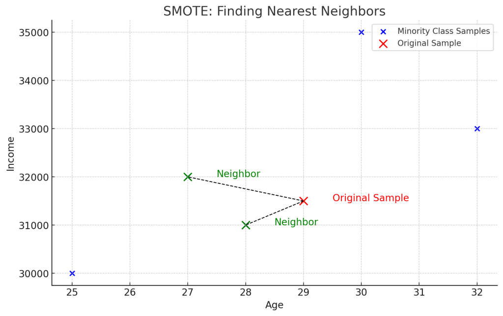
SMOTE works only by examining the minority class. It first selects a minority class data point and then finds its nearest neighbors. These neighbors are selected from within the minority class as well. For each data point in the minority class:

• SMOTE looks at the features (attributes) of the current minority class sample.
• It finds the k-nearest neighbors of this sample among other minority class samples.

Here, k is the number of neighbors selected. Typically, SMOTE uses the Euclidean distance to measure similarity between samples, but other distance metrics can also be used.

Example: Suppose you have a dataset with features representing different characteristics of people (like age, income, etc.). If you’re trying to classify rare cases of a disease (minority class), SMOTE will first identify a few people in the minority class who have similar features.

STEP 2: Generating Synthetic Samples

After finding the k-nearest neighbors, SMOTE randomly selects one neighbor from this group. It then creates a new synthetic sample by interpolating between the current sample and the selected neighbor. This means generating a new data point that lies somewhere between the two existing data points in the feature space.

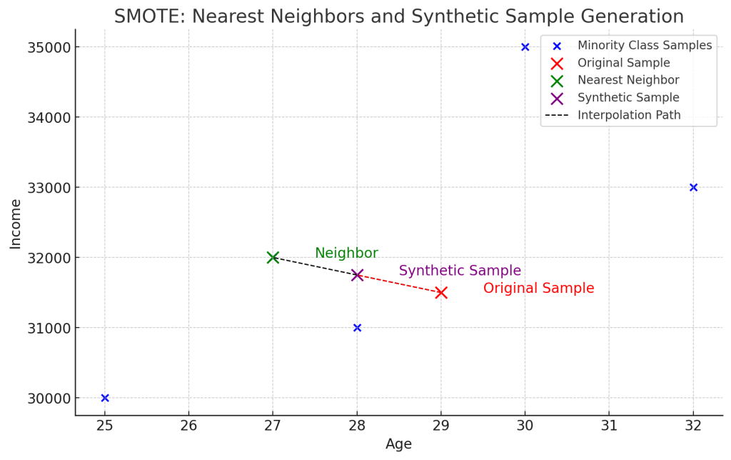
The interpolation is done using the following formula:

Where:

• x_original is the feature vector of the current minority class sample.
• x_neighbor is the feature vector of one of its nearest neighbors.
• λ is a random number between 0 and 1, so the new point will lie somewhere between the two samples.

Example:

Let’s say you have two examples in the minority class:

• Example 1: (Age: 25, Income: $30,000)
• Example 2: (Age: 30, Income: $35,000)

SMOTE might generate a synthetic example by taking a random value between these two points. If λ=0.5, the new synthetic sample will be:

• (Age: 27.5, Income: $32,500)

For detailed explanations on how SMOTE works and how to apply SMOTE in Python, check out our book Machine Learning with Imbalanced Data.

STEP 3: Repeat Until the Dataset is Balanced

SMOTE repeats the process explained in the previous step for each sample in the minority class, creating synthetic samples until the minority class has the same number of samples as the majority class (or reaches a predefined ratio).

Example of How SMOTE Balances a Dataset

Original Dataset:

• Majority Class: 100 samples
• Minority Class: 20 samples

If we apply SMOTE with a sampling ratio of 1:1, the algorithm will generate 80 synthetic minority samples, so the new dataset will have:

• Majority Class: 100 samples
• Minority Class: 100 samples (20 original + 80 synthetic)

Now we have a balanced dataset.

Implementing SMOTE in Python

Let’s take a look at how we can implement the SMOTE algorithm in Python. For this demo, we will use a dataset from Kaggle. We will first train a classifier on the imbalanced dataset to have the baseline performance, and then train it on a balanced dataset created by applying SMOTE. We will then compare the performance of both models and draw conclusions about SMOTE.

For this demo, we will be using SMOTE for binary classification, though it can also be applied to multi-class problems.

Download and Load the Dataset

You can directly download the dataset from Kaggle. It consists of numerical features representing credit card transactions. This dataset is highly imbalanced, with the majority of transactions being legitimate and only a small fraction being fraudulent. For this binary classification problem we have:

• The majority class (label 0) represents legitimate transactions.
• The minority class (label 1) represents fraudulent transactions.

Let’s go ahead and load the dataset:

import pandas as pd

# Load the dataset as pandas dataframe
df = pd.read_csv('creditcard.csv')

# Display the class distribution
print(df['Class'].value_counts())

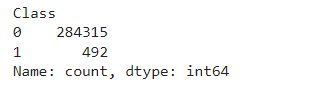
In the following image we see the number of observations for each class:

Data preprocessing

Lets split the data into features (X) and target (y), and after that, into training set and test set. To do this, we will utilize scikit-learn:

from sklearn.model_selection import train_test_split

# Separate features (X) and target (y)
X = df.drop('Class', axis=1)
y = df['Class']

# Split the dataset into training and testing sets
# (70% train, 30% test)
X_train, X_test, y_train, y_test = train_test_split(
    X, y, test_size=0.3, random_state=42, stratify=y
)

Train a Classifier on the Imbalanced Dataset

Now, lets train a classification model on the imbalanced dataset and evaluate its performance. We’ll use a Random Forest classifier:

from sklearn.ensemble import RandomForestClassifier
from sklearn.metrics import classification_report

# Train a Random Forest classifier on the imbalanced dataset
clf = RandomForestClassifier(random_state=42)
clf.fit(X_train, y_train)

# Predict on the test set
y_pred = clf.predict(X_test)

# Evaluate the model
print("Classification Report (Before SMOTE):")
print(classification_report(y_test, y_pred))

The following figure shows the classification report of the random forests trained with the imbalanced dataset. For the majority class, the precision, recall and the F1 score is 1.00. However, for the minority class, we see the recall is 0.76.

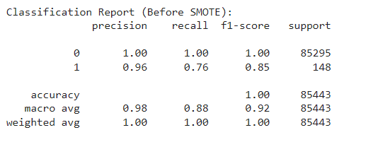
We see that the model performs better on the majority class compared to the minority class. Now, we will move on to applying SMOTE to our imbalanced dataset to create more examples of the fraudulent transactions, and see if that improves the model’s performance.

Apply SMOTE to Balance the Dataset

We will use the Python open-source library imbalanced-learn to apply SMOTE. With SMOTE, we aim to create synthetic samples for the minority class and balance the dataset.

With imbalance-learn, we have the flexibility to adjust the number of minority class samples that we want to create, by modifying the sampling_strategy parameter, which specifies the desired ratio of the minority class relative to the majority class. It can have a float value from 0 to 1.

For example, a value of 0.5 means the minority class will have half as many samples as the majority class after resampling. By default its value is set to 1, which means that the minority class will have the same number of samples as the majority class after the oversampling.

from imblearn.over_sampling import SMOTE

# Apply SMOTE to the training data
smote = SMOTE( sampling_strategy = 1.0, random_state=42)
X_resampled, y_resampled = smote.fit_resample(
    X_train, y_train)

# Check the class distribution after applying SMOTE
print(pd.Series(y_resampled).value_counts())

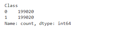
In the following figure, we can see that both classes have equal number of samples, i.e. 199020, after applying SMOTE.

Train the Classifier on the SMOTE-Augmented Dataset

We’ll train a Random Forest classifier using the SMOTE-balanced training data so that we can analyse the difference.

# Train the classifier on the SMOTE-balanced dataset
clf_smote = RandomForestClassifier(random_state=42)
clf_smote.fit(X_resampled, y_resampled)

# Predict on the test set
y_pred_smote = clf_smote.predict(X_test)

# Evaluate the model
print("Classification Report (After SMOTE):")print(
    classification_report(y_test, y_pred_smote))

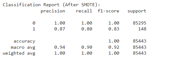
The following figure shows the classification report of the model trained with the balanced dataset. We can see that the recall for the minority class has improved from 0.76 to 0.80.

SMOTE worked! Did it?

Do you notice something wrong with how I evaluated the effectiveness of SMOTE? Exactly! Precision, recall, and F1-score are metrics that depend on the threshold, and here I am using the default classification threshold of 0.5, which is not suitable for imbalanced datasets. In fact, if we changed the threshold, we’d see different values for these metrics.

Since SMOTE generates synthetic samples, it might seem like it improves the model’s performance. But if we don’t carefully choose the right threshold for classifying the minority class, the perceived improvements could be exaggerated.

Instead of relying on the default threshold (0.5), you can adjust the threshold based on the specific use case. For example, if missing a minority class prediction is very costly like in our fraud detection example, we may want to lower the threshold to capture more instances of the minority class, and that would increase the value of recall, at the expense of precision of course. But that was the case with SMOTE anyways. There is always a trade-off between these metrics.

For a thorough discussion on whether SMOTE works, check out our YouTube video (and subscribe to stay up to date!):

If you prefer reading, then check out our imbalanced datasets article.

Comparing the classification reports

The comparison between the Classification Reports (before and after SMOTE) highlights the improvement in performance on the minority class after applying SMOTE:

Before SMOTE:

• Precision (Class 1 – Fraudulent): 0.96
• Recall (Class 1 – Fraudulent): 0.76
• F1-Score (Class 1 – Fraudulent): 0.85

In this case, while precision is high, the recall is lower (0.76), indicating that the model struggles to identify a large portion of actual fraudulent transactions. This can be problematic in scenarios like fraud detection, where missing fraudulent cases is costly.

After SMOTE:

• Precision (Class 1 – Fraudulent): 0.87
• Recall (Class 1 – Fraudulent): 0.80
• F1-Score (Class 1 – Fraudulent): 0.83

After applying SMOTE, the recall has improved from 0.76 to 0.80, meaning the model is now better at detecting more fraudulent transactions. There is a slight decrease in precision, but the overall F1-score is balanced.

SMOTE has helped the model better identify the minority class (fraudulent transactions), increasing its ability to detect fraud cases. This is how the success of SMOTE was proclaimed for years. And don’t get me wrong, it does work, under very specific circumstances. But we could have achieved the same effect by lowering the decision threshold used to classify an observation as a member of the minority class, and we would have obtained a very similar effect.

Bottom Line

• When working with imbalanced datasets, try to use strong classifiers like xgboost and lightGBMs.
• Always adjust the probability threshold used to classify an observation as a member of the minority class.
• Even small changes in recall or precision can be meaningful, especially in imbalanced domains like fraud detection, where each percentage point translates into catching more fraud.
• SMOTE is useful, but it’s probably not your first line of action when working with imbalanced datasets.

Displaying the Confusion Matrices

For the sake of the discussion, let’s continue comparing the performance of the models trained with and without data rebalancing through SMOTE.

Now lets display the confusion matrix for both models, i.e. those trained before applying SMOTE and after applying SMOTE:

from sklearn.metrics import confusion_matrix
import seaborn as sns
import matplotlib.pyplot as plt

# Confusion matrix before SMOTE with blue theme
cm_before = confusion_matrix(y_test, y_pred)
plt.figure(figsize=(6, 4))
sns.heatmap(cm_before, annot=True, fmt='d', cmap='Blues', cbar=False, linewidths=0.5)
plt.title("Confusion Matrix (Before SMOTE)")
plt.show()

# Confusion matrix after SMOTE with blue theme
cm_after = confusion_matrix(y_test, y_pred_smote)
plt.figure(figsize=(6, 4))
sns.heatmap(cm_after, annot=True, fmt='d', cmap='Blues', cbar=False, linewidths=0.5)
plt.title("Confusion Matrix (After SMOTE)")
plt.show()

Want to know how to correctly evaluate your imbalanced datasets? Check out our book Machine Learning with Imbalanced Data – clear explanations, practical python implementations.

Overall Impact

• More Fraud Caught at the Default Threshold: The model flags more fraudulent transactions after SMOTE, because the decision boundary shifted toward the minority class — not because the model got better at telling fraud apart from legitimate transactions.
• Slight Trade-off: There’s a small increase in false positives (legitimate transactions incorrectly flagged as fraud), but this is often acceptable in scenarios like fraud detection, where catching fraud is critical.

Note that the classification report is also threshold dependent, so we could have achieved the same effect shown with SMOTE, by simply changing the classification threshold used to examine the model trained on the imbalanced dataset.

Advantages of SMOTE

1. Shifts the Decision Boundary Toward the Minority Class: By balancing the classes, the prediction model flags more of the minority class at the default threshold — the same trade-off you’d get by adjusting the classification threshold on the original, imbalanced data.
2. Avoids Overfitting: Unlike random oversampling, where we duplicate existing minority samples, SMOTE generates synthetic samples. This helps avoid overfitting because the new samples are not exact copies of the original samples.
3. Works Well with weak Classifiers: SMOTE can be combined with various machine learning algorithms (such as Random Forest, Logistic Regression, SVM) and has been shown to have a bigger effect on threshold-dependent metrics for these weaker models than for strong classifiers like XGBoost.

Limitations of SMOTE

1. Synthetic Samples May Not Always Be Meaningful: SMOTE generates new data points based on linear interpolation between existing points. If the feature space has complex relationships, the synthetic samples might not represent realistic or meaningful data.
2. Overlapping Classes: If the boundary between classes is unclear (i.e., if some minority class points are too close to the majority class points), SMOTE might generate synthetic samples that actually belong to the majority class region, leading to misclassification. To address this issue we can use variations of SMOTE, such as Borderline SMOTE or Adasyn.
3. Not Suitable for Categorical Data: SMOTE works by interpolating numerical features. It doesn’t handle categorical data well. Variations of SMOTE, such as SMOTE-NC (for Nominal and Continuous data), have been developed to address this issue.

Conclusion

In this article, we learned how SMOTE (Synthetic Minority Over-sampling Technique) helps address imbalanced datasets by generating synthetic samples for the minority class. By applying SMOTE, we increased the prediction model’s recall for detecting fraudulent transactions at the default threshold — the same trade-off we could have gotten by adjusting the classification threshold on the model trained on the original data, without resampling anything. SMOTE can still be a useful, low-effort way to make cost-sensitive decisions without manually tuning a threshold, but it has limitations, and it has been shown to have the most noticeable effect in fairly specific situations: when training weak learners and evaluating with threshold-dependent metrics at the default probability threshold of 0.5.

Other ways to work with imbalanced datasets

Within the realm of data resampling, we discussed SMOTE which is an oversampling method, the alternative is to use undersampling methods to remove excessive number of majority examples.

To steer away from rebalancing, we could simply use cost-sensitive learning, or specific ensemble methods that have been designed for imbalanced datasets, like BalancingCascade or Balanced random forests.

For more details, check out our book Machine Learning with Imbalanced Data.