Isotonic Regression: A Complete Guide With Python Examples

Isotonic regression is a regression method that fits a monotonic function to data. The only thing it assumes is that, as the input increases, the output should never decrease. That single assumption makes isotonic regression surprisingly useful.

In machine learning, its most popular application is probability calibration: turning the raw scores of a classifier into probabilities we can trust, so that when the model says 70%, the event actually happens 70% of the time.

In this article, we will explore the following:

• What isotonic regression is
• How to calculate it using the pool adjacent violators algorithm (PAVA)
• How to fit an isotonic regression in Python with scikit-learn
• How to use isotonic regression to calibrate the probabilities of a classifier
• When to choose isotonic regression over Platt scaling

Isotonic regression and probability calibration are covered in depth, with Python code, in my book Imbalanced Data: Myths, Mistakes and Modern Solutions.

What Is Isotonic Regression?

Isotonic regression is a method to find the monotonically increasing function that sits as close as possible to the observed data. “Isotonic” means order preserving: if one input is larger than another, its fitted value must be larger or equal.

Isotonic regression is a non-parametric method. Beyond the order, it makes no assumption about the shape of the relationship, which can be a line, a curve, or anything in between. That makes it more flexible than linear regression, which can only fit a straight line.

The result is a non-decreasing step function, also called a piecewise constant function. The fitted values stay flat over a range of inputs, then jump up, stay flat again, and so on.

Isotonic Regression: Calculation

Suppose we have \(n\) observations, each with an input value \(x_i\) and a target \(y_i\), sorted by \(x\) from lowest to highest. Isotonic regression is a least squares problem: it looks for the fitted values \(\hat{y}_i\) that minimize the weighted sum of squared differences to the observed targets:

\[\begin{aligned} & \min_{\hat{y}} \sum_{i=1}^{n} w_i \left( y_i - \hat{y}_i \right)^2 \\ & \text{subject to} \quad \hat{y}_1 \le \dots \le \hat{y}_n \end{aligned}\]

Here, \(w_i\) is an optional weight for each observation, which is 1 when all observations count equally.

The constraint at the bottom is the monotonic constraint: each fitted value must be greater than or equal to the one before it. The constraint forces neighboring fitted values to share a common value whenever the data goes “the wrong way,” and that is what produces the steps.

How do we fit an isotonic regression?

The Pool Adjacent Violators Algorithm (PAVA)

The pool adjacent violators algorithm, PAVA or PAV for short, is the standard solver for isotonic regression. It always finds the optimal solution and, once the data is sorted, it runs in linear time.

PAVA starts with each observation as its own block, and sweeps from left to right. Whenever it finds a violation, that is, a block whose fitted value is lower than the block to its left, it pools the two blocks into one and replaces their values with their weighted average.

Sometimes, the merged block ends up lower than the block before it, creating a new violation. PAVA then keeps merging leftward until monotonicity is restored, so the final fitted values never decrease.

The PAV Algorithm Step by Step, With Numbers

Let’s work through a small example with eight observations, already sorted. To connect it with probability calibration, think of the input as a model score and the target as the observed outcome, where 1 means the event happened and 0 means it did not:

Score	Outcome
0.1	0
0.2	1
0.3	0
0.4	0
0.5	1
0.6	0
0.7	1
0.8	1

Step 1. Scores 0.1 and 0.2 have outcomes 0 and 1. The values increase, so there is no violation.

Step 2. Score 0.3 has outcome 0, lower than the 1 to its left. We pool scores 0.2 and 0.3 into one block with an average of 0.5, which is still larger than 0, so we move on.

Step 3. Score 0.4 has outcome 0, lower than the 0.5 to its left. We add it to that block, which now averages (1 + 0 + 0) / 3 = 0.33.

Step 4. Score 0.5 has outcome 1, which is larger than 0.33. No violation.

Step 5. Score 0.6 has outcome 0, lower than the 1 to its left. We pool scores 0.5 and 0.6 into a block with an average of 0.5, which is still larger than 0.33.

Step 6. Scores 0.7 and 0.8 both have outcome 1. No violations, and the algorithm is done.

These are the final fitted values, which, in the context of calibration, are the calibrated probabilities:

Score	Outcome	Block	Fitted Value
0.1	0	alone	0.00
0.2	1	pooled with 0.3 and 0.4	0.33
0.3	0	pooled with 0.2 and 0.4	0.33
0.4	0	pooled with 0.2 and 0.3	0.33
0.5	1	pooled with 0.6	0.50
0.6	0	pooled with 0.5	0.50
0.7	1	alone	1.00
0.8	1	alone	1.00

The following plot shows the observed outcomes in grey and the PAVA fit in orange:

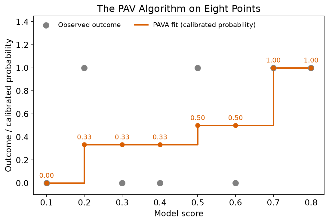
Each step is the fraction of positive outcomes among the observations it covers. Among scores 0.2, 0.3 and 0.4, one out of three was positive, so the fitted value is 0.33.

Advantages and Limitations of Isotonic Regression

As with any algorithm, isotonic regression has its strengths and weaknesses. Let’s go over them.

Advantages of Isotonic Regression

• No assumed shape: it can follow any monotonic trend.
• No hyperparameters to tune: once we choose the direction, the solution is unique.
• Fast: PAVA runs in linear time once the data is sorted, so it scales to large datasets.
• Easy to interpret: each step is the average target of a group of neighboring observations.

Limitations of Isotonic Regression

• Step-shaped fits: the fitted function is not smooth. Monotone splines are an alternative when we expect gradual changes.
• No extrapolation: new values outside the training range are clipped to the nearest step, or returned as missing.
• Sensitive to outliers: because it minimizes squared errors, a single extreme value can create or flatten a step.
• Overfitting on small datasets: with few observations, the steps follow the noise, especially at the edges of the input range.
• Requires a monotonic relationship: if the true relationship goes up and then down, isotonic regression will flatten it.

Isotonic Regression in Python With Scikit-learn

Scikit-learn implements isotonic regression in the IsotonicRegression class, which uses PAVA under the hood. Let’s create a variable that grows quickly for small values of x and then flattens, and add some noise to it:

import numpy as np
import matplotlib.pyplot as plt
from sklearn.isotonic import IsotonicRegression

rng = np.random.default_rng(42)

n = 100
x = np.arange(n)
y = 50 * np.log1p(x) + rng.integers(-50, 50, size=n)

Next, we fit the isotonic regression:

iso = IsotonicRegression(out_of_bounds="clip")
y_iso = iso.fit_transform(x, y)

The fit_transform() method learns the step function and returns the fitted values for the training data in a single call.

Let’s check that the fitted values are monotonic, and count how many steps the model learned:

print("Non-decreasing:", np.all(np.diff(y_iso) >= 0))
print("Number of steps:", len(np.unique(y_iso)))

The output confirms that the fit never goes down, and that 100 observations were summarized in 15 steps:

Non-decreasing: True
Number of steps: 15

Finally, we plot the data alongside the isotonic fit:

fig, ax = plt.subplots(figsize=(8, 5))
ax.scatter(x, y, s=18, color="grey", alpha=0.6, label="Observations")
ax.plot(x, y_iso, drawstyle="steps-post", label="Isotonic regression")
ax.set_xlabel("x")
ax.set_ylabel("y")
ax.legend()
plt.show()

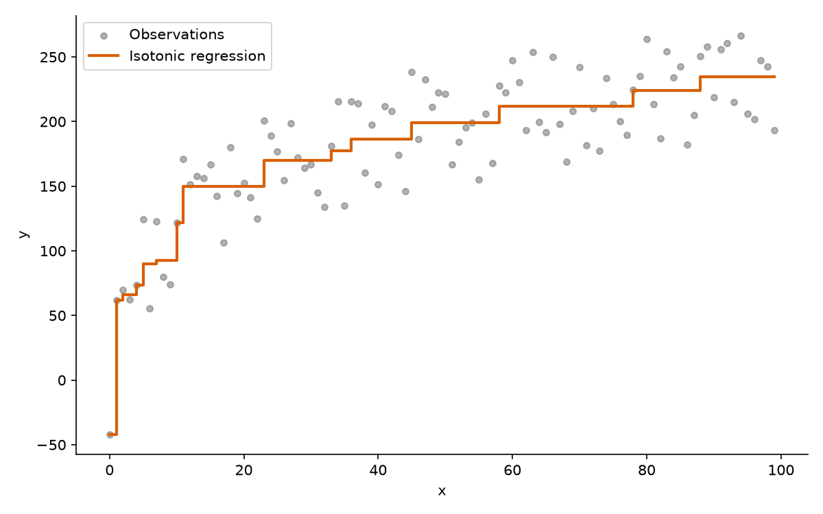
In the following plot, we see the isotonic regression following the curved trend of the data as a step function:

The Main Parameters of IsotonicRegression

IsotonicRegression has only a handful of parameters:

• increasing: whether the fitted function should be non-decreasing (True, the default) or non-increasing (False). With "auto", scikit-learn infers the direction from the data.
• out_of_bounds: what to do with new values outside the training range. The default, "nan", returns missing values, "clip" returns the fitted value of the nearest end, and "raise" throws an error.
• y_min and y_max: optional lower and upper bounds for the fitted values.

For probability calibration, out_of_bounds="clip" is usually the safest choice. With clipping, a new observation with a score slightly higher than anything in the calibration data gets the highest calibrated probability.

How IsotonicRegression Predicts New Values

Once fitted, IsotonicRegression stores the boundaries of each block in its X_thresholds_ and y_thresholds_ attributes. The predict() method is flat within a block, and interpolates linearly between adjacent blocks.

For example, in our PAVA example, a score of 0.45 falls between the block that ends at 0.4, with a value of 0.33, and the block that starts at 0.5, with a value of 0.5. It gets a prediction of 0.42.

So, strictly speaking, scikit-learn predicts with a piecewise linear function, which explains why calibrated probabilities occasionally fall between the steps of the isotonic fit.

Isotonic Regression for Probability Calibration

The best-known use of isotonic regression in machine learning is probability calibration. Let’s quickly recap what calibration is; for a broader introduction, check out our article on probability calibration in machine learning.

What Are Calibrated Probabilities?

If a model predicts a disease with a probability of 70% for one hundred patients, roughly 70 of them should actually have the disease. Probabilities with this property are called calibrated.

Many classifiers return scores that rank observations well, but do not match the real frequency of the event. A model can achieve an outstanding ROC-AUC and still produce awful probability estimates.

Assessing Calibration With Reliability Diagrams

To check whether a model is calibrated, we use a calibration curve, also known as a reliability diagram. We sort the predicted probabilities into intervals, and for each interval, we plot the average predicted probability against the fraction of observations that belong to the positive class.

A perfectly calibrated model follows the diagonal. The following reliability diagram, for a logistic regression, stays close to it:

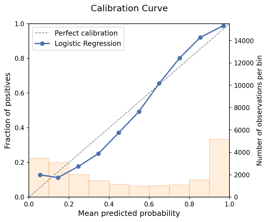
Keep in mind that reliability diagrams need plenty of data. With small or imbalanced test sets, some intervals contain only a handful of observations, and the curve can look miscalibrated purely due to noise.

Metrics like the log loss and the Brier score also reward calibrated probabilities, but they reward good ranking too. That is why the reliability diagram is the most direct way to see whether the probabilities match reality.

How Isotonic Regression Calibrates a Classifier

To fix miscalibrated probabilities, we fit a second model that takes the classifier’s scores as input and returns calibrated probabilities. The two most common choices are isotonic regression and Platt scaling, which we compare later in this article.

Isotonic regression only assumes that higher scores correspond to higher probabilities, which is what we expect from any useful classifier. Formally, given the model scores \(f_i\) and the true outcomes \(y_i\), isotonic calibration assumes:

\[y_i = m(f_i) + \varepsilon_i\]

where \(m\) is some monotonically increasing function, and \(\varepsilon_i\) is noise. Isotonic regression finds the step function that best approximates \(m\) using PAVA, exactly as in our eight observation example.

Isotonic Calibration Needs Its Own Data

If we fit the isotonic regression on the data used to train the classifier, the calibration will look better than it really is. The ideal setup has three datasets: a training set for the classifier, a calibration set for the isotonic regression, and a test set to evaluate the calibrated pipeline.

When there is not enough data for three subsets, we can use cross-validation instead. With cv=5, scikit-learn’s CalibratedClassifierCV trains the classifier on 4 folds, fits the isotonic regression on the remaining fold, repeats this 5 times, and averages the results. In the following demo, we’ll use a dedicated calibration set, because it makes each step easier to follow.

Calibrating a Classifier With Isotonic Regression in Python

Let’s put all of this into practice. We will use the bank marketing dataset, where the goal is to predict whether a client will subscribe to a term deposit. Only about 12% of the clients subscribe, so the data is imbalanced.

We’ll train a Gaussian naive Bayes, check whether its probabilities are calibrated with a reliability diagram, and, if they are not, recalibrate them with isotonic regression.

Training the Classifier

Let’s import the modules and load the data:

import matplotlib.pyplot as plt
from feature_engine.encoding import OrdinalEncoder
from sklearn.calibration import CalibrationDisplay, CalibratedClassifierCV
from sklearn.datasets import fetch_openml
from sklearn.frozen import FrozenEstimator
from sklearn.model_selection import train_test_split
from sklearn.naive_bayes import GaussianNB
from sklearn.preprocessing import StandardScaler

SEED = 42

data = fetch_openml(
    name="bank-marketing", version=1, as_frame=True, parser="auto",
)
X = OrdinalEncoder(encoding_method="arbitrary").fit_transform(data.data)
y = (data.target == "2").astype(int)

We encode the categorical variables into numbers with Feature-engine’s OrdinalEncoder, because naive Bayes only works with numerical variables.

Now, we split the data into a training set (60%), a calibration set (20%), and a test set (20%):

X_train, X_tmp, y_train, y_tmp = train_test_split(
    X, y, test_size=0.40, random_state=SEED, stratify=y,
)

X_cal, X_test, y_cal, y_test = train_test_split(
    X_tmp, y_tmp, test_size=0.50, random_state=SEED, stratify=y_tmp,
)

Next, we scale the features, train the naive Bayes, and obtain its probabilities for the test set:

scaler = StandardScaler()
X_train_sc = scaler.fit_transform(X_train)
X_cal_sc = scaler.transform(X_cal)
X_test_sc = scaler.transform(X_test)

gnb = GaussianNB().fit(X_train_sc, y_train)
probs_raw = gnb.predict_proba(X_test_sc)[:, 1]

Checking Calibration With a Reliability Diagram

Are the probabilities of the naive Bayes calibrated? Let’s find out by plotting its reliability diagram on the test set:

fig, ax = plt.subplots(figsize=(6, 6))
CalibrationDisplay.from_predictions(
    y_test, probs_raw, n_bins=10, ax=ax, name="Naive Bayes",
)
ax.set_title("Reliability diagram: naive Bayes")
plt.show()

In the following reliability diagram, we see that the calibration curve of the naive Bayes lies far below the diagonal:

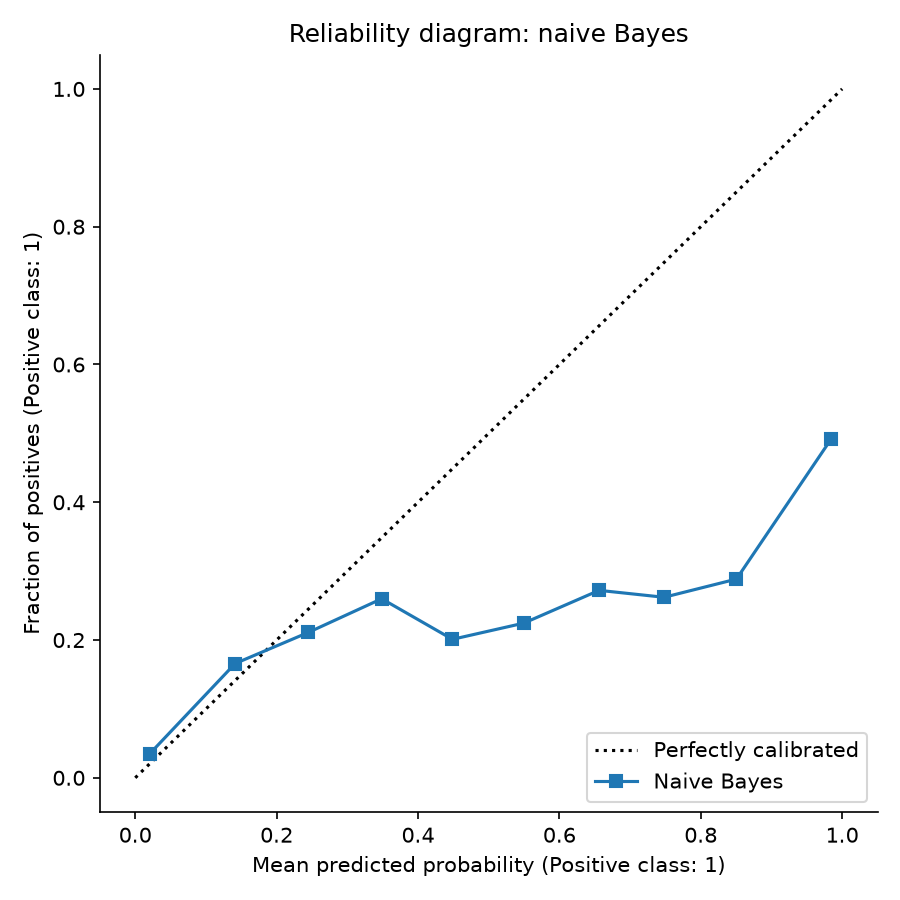
When the naive Bayes predicts a probability of 98%, only about half of those clients actually subscribe. And predictions between 40% and 90% correspond to subscription rates of only 20% to 30%.

In other words, the naive Bayes is overconfident: its probabilities are much higher than the real frequency of the event. Let’s fix that with isotonic regression.

Recalibrating the Classifier With Isotonic Regression

We fit the isotonic regression on the calibration set, and obtain the calibrated probabilities for the test set:

cal_gnb = CalibratedClassifierCV(FrozenEstimator(gnb), method="isotonic")
cal_gnb.fit(X_cal_sc, y_cal)
probs_cal = cal_gnb.predict_proba(X_test_sc)[:, 1]

FrozenEstimator tells scikit-learn that the naive Bayes is already trained, so it does not retrain it. CalibratedClassifierCV only learns how to remap its outputs to the observed frequencies of the target.

Checking Calibration After Isotonic Regression

Now, let’s plot the reliability diagram of the naive Bayes before and after isotonic calibration:

fig, ax = plt.subplots(figsize=(6, 6))
CalibrationDisplay.from_predictions(
    y_test, probs_raw, n_bins=10, ax=ax, name="Naive Bayes",
)
CalibrationDisplay.from_predictions(
    y_test, probs_cal, n_bins=10, ax=ax,
    name="Naive Bayes + isotonic regression",
)
ax.set_title("Reliability diagram: before and after isotonic calibration")
plt.show()

And voilà! After isotonic regression, the calibration curve, in orange, follows the diagonal closely:

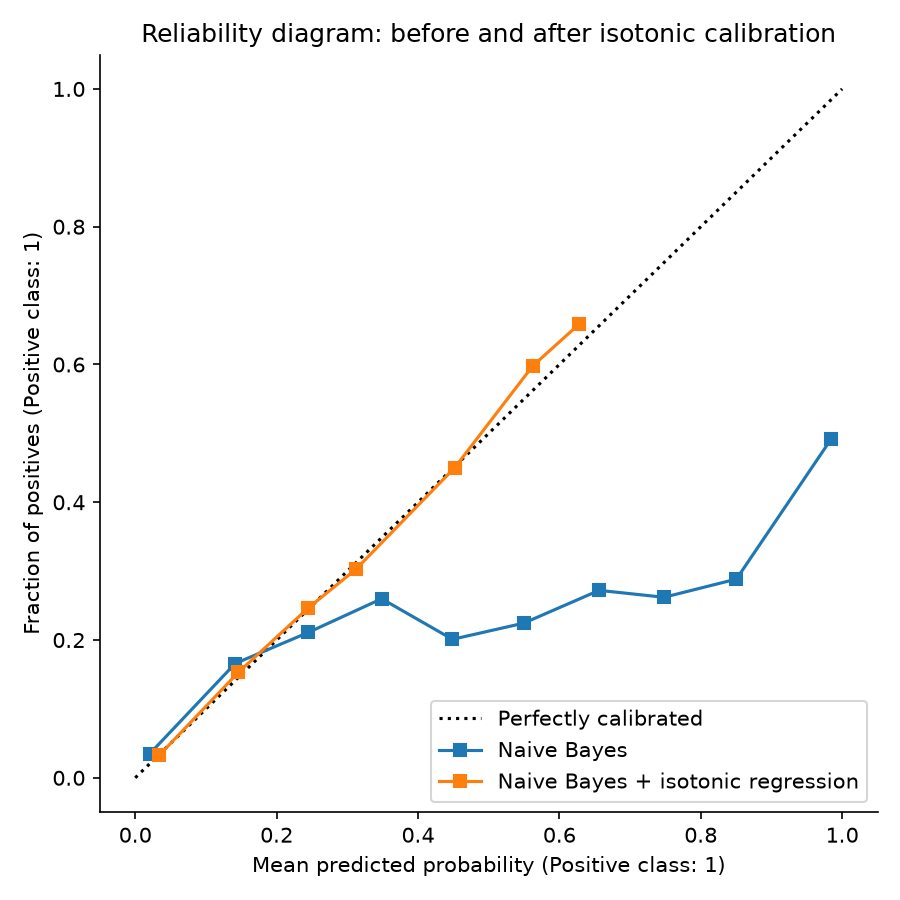
Now, when the model says that a client has a 45% chance of subscribing, about 45% of those clients actually subscribe. These are probabilities we can act on.

Notice also that the calibrated curve stops at around 0.65. Even the clients that the naive Bayes was most certain about subscribed only about 63% of the time in the calibration set, so that is the highest probability the isotonic regression returns.

Isotonic Regression vs Platt Scaling

The other popular recalibration method is Platt scaling, which passes the model scores through a sigmoid function with two parameters. Which one should we choose? It depends on the shape of the miscalibration and on how much data we have.

Platt scaling works well when the distortion in the predicted probabilities follows a sigmoid shape. Isotonic regression can correct any monotonic distortion, which makes it the better choice for models with complex calibration errors, like the naive Bayes in our demo.

On the other hand, with only two parameters, Platt scaling is hard to overfit, so it generalizes better when the calibration set is small. Isotonic regression needs more data, and in highly imbalanced datasets, there may be so few positive observations that the fitted steps become unstable.

The following table summarizes the main differences:

Property	Platt Scaling	Isotonic Regression
Mapping function	Sigmoid	Any non-decreasing step function
Parameters	2	One per step
Best when	Distortion is sigmoid shaped	Distortion has any monotonic shape
Small calibration sets	Generalizes well	Prone to overfitting
Large calibration sets	Can be too rigid	Often the most accurate
Calibrated probabilities	Smooth and continuous	Coarse, many ties

In scikit-learn, switching between the two takes a single argument, method="sigmoid" or method="isotonic", so it is easy to try both and compare them on your test set.

Train Calibrated Classifiers Instead

Before we wrap up, I want to stress what I think is the most important message of this article. Isotonic regression does a great job at fixing probabilities, but fixing calibration means training a second model at the back of our classifier.

And that second model comes with all the responsibilities of any model. It needs its own data, which we take away from training the classifier, and its own evaluation on a test set, to make sure the calibration generalizes. Every time we retrain the classifier, we need to recalibrate it too.

So, whenever possible, train classifiers that return calibrated probabilities in the first place. Choose models that optimize the log loss, like logistic regression or gradient boosting machines, and tune them with proper scoring rules like the log loss or the Brier score.

Avoid class weights and resampling methods like SMOTE, because they change the class balance the model learns from and distort its probabilities, as we discuss in our article on machine learning with imbalanced data. Use isotonic regression when, after all that, the probabilities still do not match reality.

Wrap-Up

Isotonic regression fits the best possible monotonic function to the data, without assuming any particular shape, and the pool adjacent violators algorithm solves it efficiently.

In machine learning, isotonic regression shines as a probability calibration method. It preserves the ranking of the classifier while turning its scores into probabilities that match the real frequency of the event. Fit it on data the classifier has not seen, and prefer Platt scaling when the calibration set is small.

Above all, remember that recalibration means training and evaluating another model. Train calibrated classifiers whenever you can, and keep isotonic regression for when you need it.

If you want to go deeper into probability calibration, proper scoring rules, and why resampling and class weights distort probabilities, check out my book Imbalanced Data: Myths, Mistakes and Modern Solutions.

References

• Niculescu-Mizil and Caruana. 2005. Predicting Good Probabilities With Supervised Learning. Proceedings of the 22nd International Conference on Machine Learning.
• Fawcett and Niculescu-Mizil. 2007. PAV and the ROC Convex Hull. Machine Learning.