Confusion Matrix, Precision, and Recall: A Complete Guide With Python Examples

A confusion matrix is a table that shows how many predictions of a classification model were correct and how many were wrong, broken down by class. Precision tells us how many of the positive predictions were correct, and recall tells us how many of the actual positives the model found.

Together, the confusion matrix, precision and recall are the starting point to evaluate any classifier. They tell us much more than accuracy alone, especially when the data is imbalanced.

In this article, we will explore the following:

• What a confusion matrix is and how to read it
• How to calculate accuracy, precision, recall and the F1 score from the confusion matrix
• The precision vs recall trade-off, and how the decision threshold controls it
• Other metrics we can derive from the confusion matrix, like specificity
• How to compute the confusion matrix, precision and recall in Python with scikit-learn
• How the confusion matrix works for multiclass classification

Classification metrics, and how to choose them when the data is imbalanced, are covered in depth in my book Imbalanced Data: Myths, Mistakes and Modern Solutions.

What Is a Confusion Matrix?

A confusion matrix compares the labels predicted by a machine learning model with the actual labels of the data. Each cell counts how many observations fall into one combination of actual and predicted class.

In binary classification, we have two classes. We call the class we want to detect the positive class, like spam, fraud or disease, and the other one the negative class.

With two classes, there are four possible outcomes for each prediction, so the confusion matrix is a 2x2 table.

True Positives, False Positives, True Negatives and False Negatives

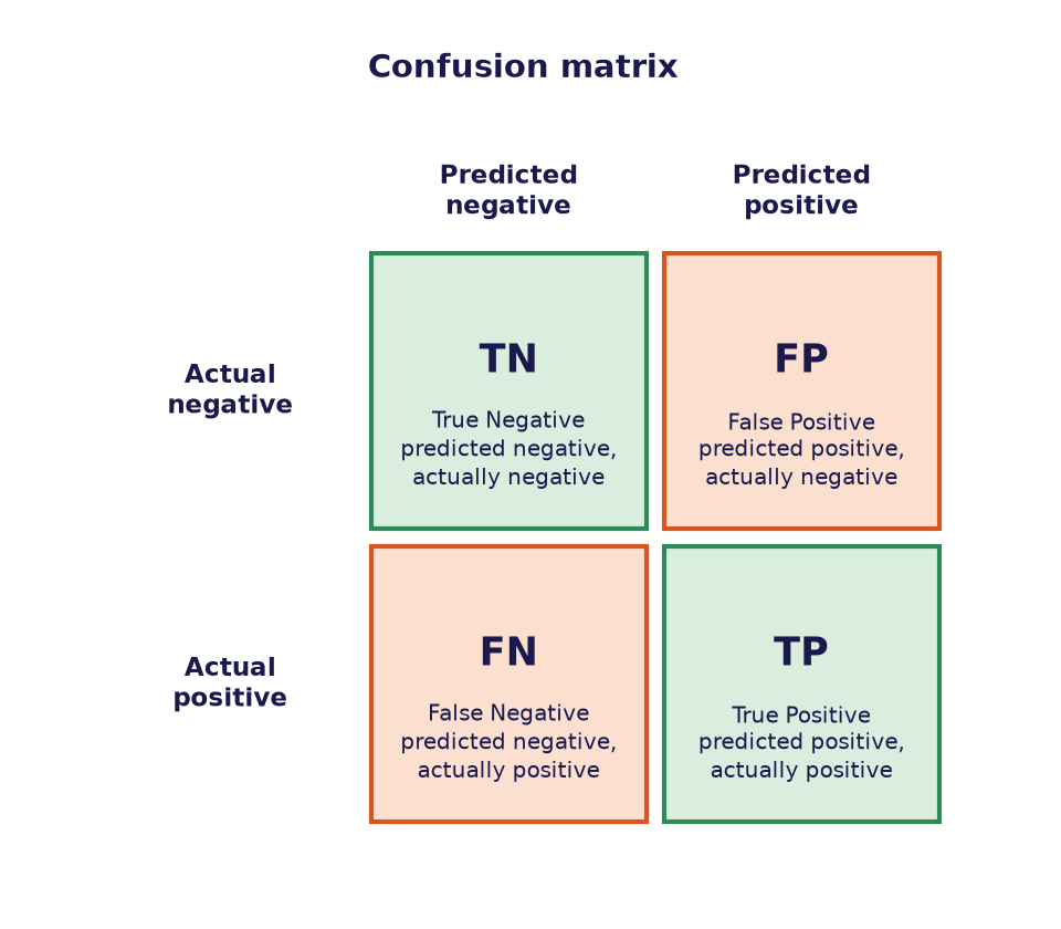
These are the four outcomes:

• True Positive (TP): the model predicted positive, and the observation is actually positive.
• False Positive (FP): the model predicted positive, but the observation is actually negative.
• True Negative (TN): the model predicted negative, and the observation is actually negative.
• False Negative (FN): the model predicted negative, but the observation is actually positive.

The following diagram shows where each outcome sits in the confusion matrix. The green cells are the correct predictions, and the orange cells are the errors:

How to Read a Confusion Matrix

In this article, the rows show the actual labels and the columns show the predicted labels. This is the layout scikit-learn uses, with the negative class first, so the true negatives sit in the top left corner and the true positives in the bottom right.

Be aware that some books and tools swap rows and columns. Before interpreting a confusion matrix, always check which axis shows the actual labels and which shows the predictions.

A simple trick helps to remember the names. The second word, positive or negative, is what the model predicted, and the first word, true or false, tells us whether that prediction was correct.

Type I and Type II Errors

The two kinds of mistakes have names borrowed from statistics. A false positive is a type I error, a false alarm. A false negative is a type II error, a miss.

Which error is worse depends on the problem. Missing a disease is usually worse than a false alarm, while sending an important email to the spam folder can be worse than letting one spam message through.

Confusion Matrix Example: A Spam Filter

Let’s make this concrete. Suppose we have a spam filter, and we use it to classify 1,000 emails, of which 100 are spam and 900 are legitimate.

The filter correctly flags 80 of the 100 spam emails, and lets the other 20 into the inbox. It also sends 40 legitimate emails to the spam folder by mistake, and correctly delivers the remaining 860.

This is the confusion matrix of our spam filter:

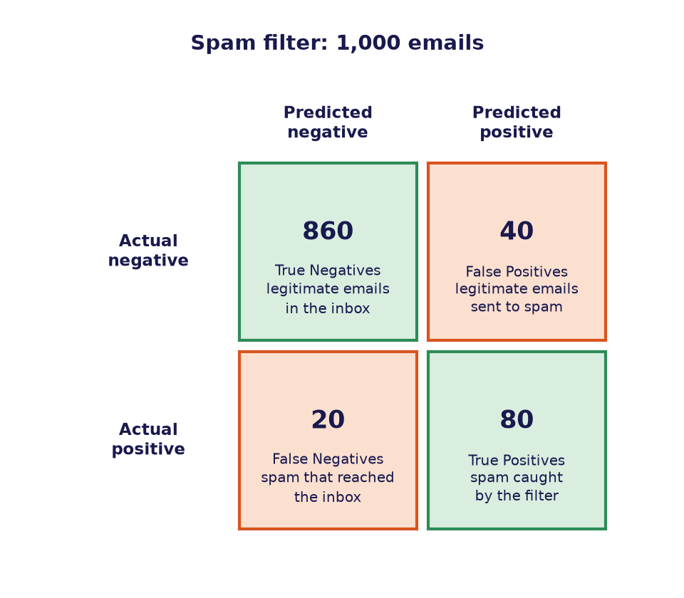
Notice that each row adds up to the actual number of emails in that class: 860 + 40 = 900 legitimate emails, and 20 + 80 = 100 spam emails. This is a quick sanity check whenever you build a confusion matrix by hand.

We will use these numbers to calculate every metric in the following sections.

Accuracy From the Confusion Matrix

Accuracy is the fraction of predictions that the model got right. We obtain it by adding the correct predictions on the diagonal of the confusion matrix and dividing by the total:

\[\text{Accuracy} = \frac{TP + TN}{TP + TN + FP + FN}\]

For our spam filter, the accuracy is (80 + 860) / 1,000 = 0.94, or 94%. That sounds great, but accuracy hides an important problem.

The Accuracy Paradox on Imbalanced Data

Imagine a lazy spam filter that labels every email as legitimate. It would never catch a single spam message, yet its accuracy would be 900 / 1,000 = 90%.

This is known as the accuracy paradox. When one class is much more frequent than the other, a model can reach a high accuracy just by predicting the majority class, as we discuss in our article on class imbalance in machine learning.

To find out how well the model handles the positive class, we need metrics that look at the errors separately. That’s where precision and recall come in.

Precision: How Many Positive Predictions Are Correct?

Precision answers the question: of all the observations that the model predicted as positive, how many are actually positive? In our example, when the spam filter flags an email as spam, how often is it right?

Precision Formula

Precision is the number of true positives divided by all positive predictions, that is, the true positives plus the false positives:

\[\text{Precision} = \frac{TP}{TP + FP}\]

Our spam filter flagged 80 + 40 = 120 emails as spam, and 80 of them were actually spam. So, the precision is 80 / 120 = 0.67.

In other words, one in three emails in the spam folder is a legitimate email that the user may never see. Precision is also known as the positive predictive value.

When Precision Matters

Precision is the metric to watch when false positives are costly. In spam detection, a false positive means a missed job offer or an unpaid invoice.

Other examples are recommending products, where irrelevant suggestions annoy customers, and fraud detection systems that block cards, where every false alarm stops a legitimate customer from paying.

Recall: How Many Positives Does the Model Find?

Recall answers a different question: of all the observations that are actually positive, how many did the model find? In our example, out of all the spam emails, how many did the filter catch?

Recall Formula

Recall is the number of true positives divided by all actual positives, that is, the true positives plus the false negatives:

\[\text{Recall} = \frac{TP}{TP + FN}\]

There were 80 + 20 = 100 spam emails, and the filter caught 80 of them. So, the recall is 80 / 100 = 0.80.

Recall is also known as sensitivity, true positive rate or hit rate. You will find all these names in the literature, and they all mean the same thing.

When Recall Matters

Recall is the metric to watch when false negatives are costly. In medical diagnosis, a false negative means a sick patient who goes home without treatment.

The same applies to fraud detection, where every missed fraudulent transaction is money lost, and to defect detection in manufacturing, where a missed defect reaches the customer.

Precision and Recall in the Confusion Matrix

A visual way to remember the difference between precision and recall is to look at which cells of the confusion matrix each one uses. Both have the true positives in the numerator, but they divide by different totals.

Precision divides by the predicted positive column, while recall divides by the actual positive row:

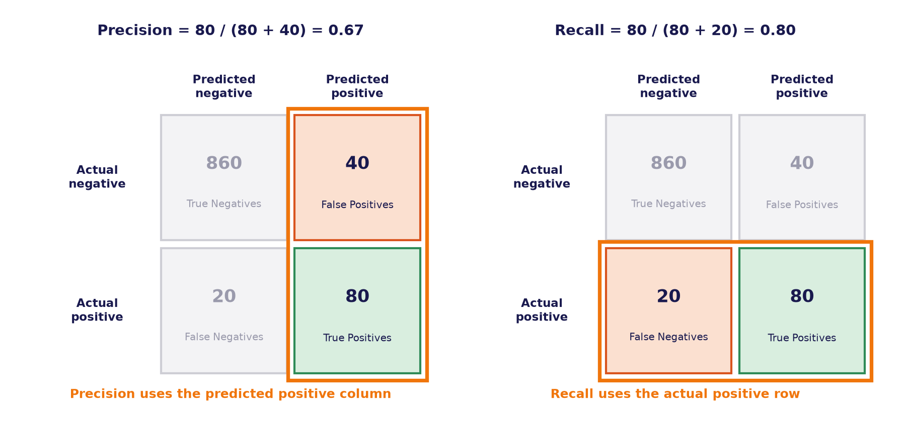
Notice also that neither precision nor recall uses the true negatives. That is why they are so useful on imbalanced data: the large number of easy negatives cannot inflate them the way it inflates accuracy.

Precision vs Recall: The Trade-off

Most classifiers return a score or probability for each observation, which we turn into a class with a decision threshold. By default, this threshold is usually 0.5.

If we lower the threshold, the model labels more observations as positive. It catches more of the actual positives, so recall goes up, but it also raises more false alarms, so precision usually goes down.

If we raise the threshold, the opposite happens: the model only flags the observations it is most certain about, so precision goes up and recall goes down. We will see this with real numbers in the Python demo.

Choosing Between Precision and Recall

There is no universal answer to which metric is more important. It depends on the cost of each error in your application.

A cancer screening test should favor recall, because a false alarm leads to more tests, while a miss can cost a life. A spam filter should favor precision, because users prefer deleting a few spam emails to losing an important one.

To see the trade-off at every threshold at once, we can plot a precision-recall curve. We cover it in depth in our article on precision-recall curves.

F1 Score: Combining Precision and Recall

Sometimes we want a single number that summarizes both precision and recall, for example to compare models. The F1 score does exactly that, by taking the harmonic mean of the two:

\[F_1 = 2 \times \frac{\text{Precision} \times \text{Recall}}{\text{Precision} + \text{Recall}}\]

For our spam filter, the F1 score is 2 × (0.67 × 0.80) / (0.67 + 0.80) = 0.73.

Why the Harmonic Mean?

The harmonic mean punishes low values more than the regular average. A model with a precision of 1.0 and a recall of 0.1 has an average of 0.55, but an F1 score of only 0.18, which better reflects that the model misses most positives.

When one of the two metrics matters more than the other, we can use the F-beta score instead. With beta greater than 1 it gives more weight to recall, and with beta smaller than 1 it gives more weight to precision.

Specificity and Other Metrics From the Confusion Matrix

Precision and recall focus on the positive class. The confusion matrix also lets us calculate metrics that describe how the model handles the negative class.

The most common one is specificity, also called the true negative rate. It tells us what fraction of the actual negatives the model labeled correctly:

\[\text{Specificity} = \frac{TN}{TN + FP}\]

The table below summarizes the main metrics we can derive from the confusion matrix, with their values for our spam filter:

Metric	Also known as	Formula	Spam filter
Accuracy		(TP + TN) / total	0.94
Precision	Positive predictive value	TP / (TP + FP)	0.67
Recall	Sensitivity, true positive rate	TP / (TP + FN)	0.80
Specificity	True negative rate	TN / (TN + FP)	0.96
False positive rate	1 minus specificity	FP / (FP + TN)	0.04
False negative rate	1 minus recall	FN / (FN + TP)	0.20
F1 score		2TP / (2TP + FP + FN)	0.73

The true positive rate and the false positive rate are the two axes of the ROC curve, which we discuss in our article on AUC-ROC analysis. Recall and specificity together give us the balanced accuracy, an alternative to accuracy for imbalanced data.

Confusion Matrix, Precision and Recall in Python With Scikit-learn

Let’s now compute all of this in Python. We will use the bank marketing dataset, where the goal is to predict whether a client will subscribe to a term deposit after a marketing call.

Only about 12% of the clients subscribe, so the data is imbalanced, just like in many real classification problems.

Training a Classification Model

Let’s import the libraries and load the data:

import numpy as np
import pandas as pd
import matplotlib.pyplot as plt
from feature_engine.encoding import OneHotEncoder
from sklearn.datasets import fetch_openml
from sklearn.linear_model import LogisticRegression
from sklearn.metrics import (
    ConfusionMatrixDisplay,
    accuracy_score,
    classification_report,
    confusion_matrix,
    f1_score,
    precision_score,
    recall_score,
)
from sklearn.model_selection import train_test_split
from sklearn.pipeline import make_pipeline
from sklearn.preprocessing import StandardScaler

data = fetch_openml(
    name="bank-marketing", version=1, as_frame=True, parser="auto",
)
X = data.data
y = (data.target == "2").astype(int)

The target is 1 when the client subscribed, the positive class, and 0 otherwise. Next, we split the data into a training set and a test set:

X_train, X_test, y_train, y_test = train_test_split(
    X, y, test_size=0.3, random_state=42, stratify=y,
)

Now, we train a logistic regression. We put it in a pipeline with Feature-engine’s OneHotEncoder, to encode the categorical variables, and a StandardScaler:

model = make_pipeline(
    OneHotEncoder(drop_last=True),
    StandardScaler(),
    LogisticRegression(max_iter=1000),
)
model.fit(X_train, y_train)

y_pred = model.predict(X_test)

The predict() method returns the predicted class for each client in the test set, using the default threshold of 0.5.

Computing the Confusion Matrix With Scikit-learn

To obtain the confusion matrix, we pass the actual and predicted labels to scikit-learn’s confusion_matrix() function:

cm = confusion_matrix(y_test, y_pred)
print(cm)

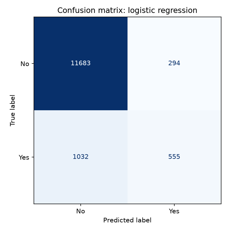
The output is a NumPy array, with the actual labels in the rows and the predicted labels in the columns:

[[11683   294]
 [ 1032   555]]

For binary classification, we can unpack the four values with ravel(). Remember that scikit-learn puts the negative class first:

tn, fp, fn, tp = cm.ravel()
print(f"TN={tn}, FP={fp}, FN={fn}, TP={tp}")

TN=11683, FP=294, FN=1032, TP=555

Plotting the Confusion Matrix

An array is hard to read, so let’s plot the confusion matrix with ConfusionMatrixDisplay:

fig, ax = plt.subplots(figsize=(5, 5))
ConfusionMatrixDisplay.from_predictions(
    y_test,
    y_pred,
    display_labels=["No", "Yes"],
    cmap="Blues",
    colorbar=False,
    ax=ax,
)
ax.set_title("Confusion matrix: logistic regression")
plt.show()

In the following plot, we see that the model identified most clients who did not subscribe correctly, but missed 1,032 of the 1,587 clients who did:

Calculating Precision, Recall and F1 Score in Python

Scikit-learn has a function for each metric. They all take the actual and predicted labels:

print("Accuracy: ", round(accuracy_score(y_test, y_pred), 3))
print("Precision:", round(precision_score(y_test, y_pred), 3))
print("Recall:   ", round(recall_score(y_test, y_pred), 3))
print("F1 score: ", round(f1_score(y_test, y_pred), 3))

This is what we get:

Accuracy:  0.902
Precision: 0.654
Recall:    0.35
F1 score:  0.456

Here we see the accuracy paradox in action. The accuracy is 90%, but a model that always predicts “No” would already reach 88%, because that is the share of clients who did not subscribe.

The recall tells the real story: the model finds only 35% of the clients who subscribe. When it does flag a client, it is right 65% of the time, which is the precision.

The Classification Report

To get precision, recall and F1 score for every class in one go, we can use classification_report():

print(classification_report(y_test, y_pred, target_names=["No", "Yes"]))

              precision    recall  f1-score   support

          No       0.92      0.98      0.95     11977
         Yes       0.65      0.35      0.46      1587

    accuracy                           0.90     13564
   macro avg       0.79      0.66      0.70     13564
weighted avg       0.89      0.90      0.89     13564

Each row shows the metrics when we treat that class as the positive one, and the support is the number of actual observations in the class. The last two rows average the metrics across classes, which we explain in the multiclass section below.

Changing the Decision Threshold

The default threshold of 0.5 gives us a low recall. Let’s see what happens to precision and recall when we change it. We obtain the probabilities with predict_proba() and apply different thresholds:

probs = model.predict_proba(X_test)[:, 1]

rows = []
for t in [0.1, 0.2, 0.3, 0.5, 0.7]:
    y_pred_t = (probs >= t).astype(int)
    rows.append({
        "threshold": t,
        "precision": precision_score(y_test, y_pred_t),
        "recall": recall_score(y_test, y_pred_t),
        "f1": f1_score(y_test, y_pred_t),
    })

print(pd.DataFrame(rows).round(3))

   threshold  precision  recall     f1
0        0.1      0.381   0.857  0.527
1        0.2      0.506   0.668  0.576
2        0.3      0.581   0.537  0.558
3        0.5      0.654   0.350  0.456
4        0.7      0.674   0.200  0.309

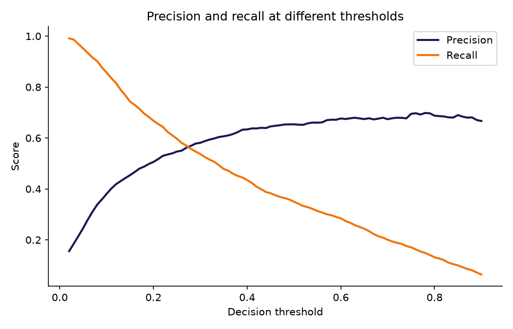
This is the precision-recall trade-off with real numbers. Lowering the threshold to 0.2 almost doubles the recall, from 0.35 to 0.67, at the price of a lower precision, and it also improves the F1 score.

Let’s plot precision and recall across many thresholds:

thresholds = np.linspace(0.02, 0.9, 89)
precision = [precision_score(y_test, (probs >= t).astype(int)) for t in thresholds]
recall = [recall_score(y_test, (probs >= t).astype(int)) for t in thresholds]

fig, ax = plt.subplots(figsize=(7, 4.5))
ax.plot(thresholds, precision, label="Precision", color="#19194e")
ax.plot(thresholds, recall, label="Recall", color="#f0750b")
ax.set_xlabel("Decision threshold")
ax.set_ylabel("Score")
ax.set_title("Precision and recall at different thresholds")
ax.legend()
plt.show()

In the following plot, we see recall falling steadily as the threshold increases, while precision rises:

The right threshold depends on the cost of each error. If calling a client who won’t subscribe is cheap, and missing one who would is expensive, a low threshold makes sense.

Confusion Matrix for Multiclass Classification

The confusion matrix also works with more than two classes. With k classes, it becomes a k x k table, where the diagonal holds the correct predictions and every other cell counts one specific type of confusion between two classes.

Let’s look at an example with a model that classifies 100 animal pictures as cats, dogs or rabbits:

y_true = ["cat"] * 50 + ["dog"] * 30 + ["rabbit"] * 20
y_pred = (
    ["cat"] * 42 + ["dog"] * 6 + ["rabbit"] * 2
    + ["cat"] * 5 + ["dog"] * 22 + ["rabbit"] * 3
    + ["cat"] * 2 + ["dog"] * 6 + ["rabbit"] * 12
)

labels = ["cat", "dog", "rabbit"]
disp = ConfusionMatrixDisplay.from_predictions(
    y_true, y_pred, labels=labels, cmap="Blues", colorbar=False,
)
disp.ax_.set_title("Multiclass confusion matrix")
plt.show()

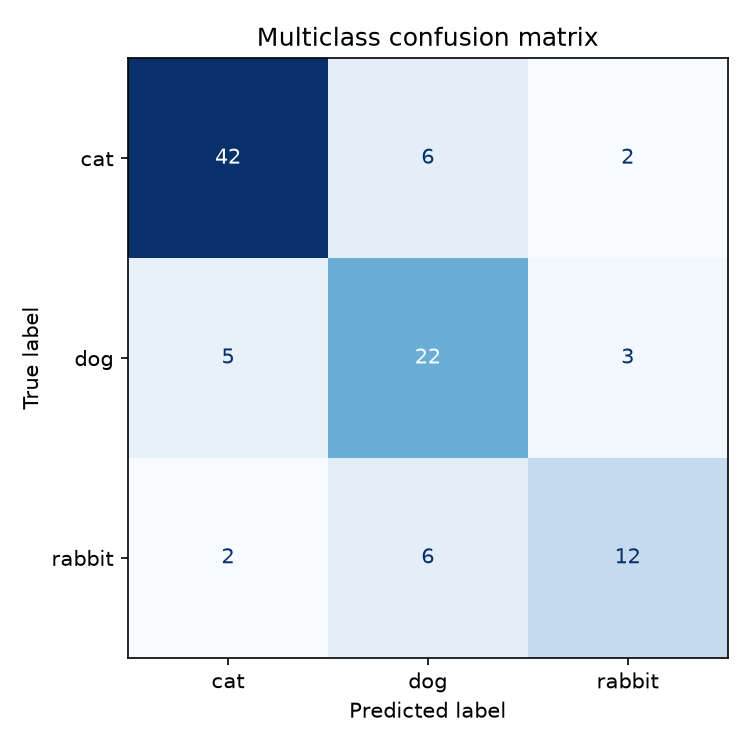
The multiclass confusion matrix shows, for example, that 6 cats were mistaken for dogs, and 6 rabbits for dogs as well:

Precision and Recall for Each Class

In multiclass classification, we calculate precision and recall for each class separately, treating that class as the positive one and all the others as negative. This is called the one-vs-rest approach.

For cats, the model predicted 42 + 5 + 2 = 49 pictures as cats, and 42 of them were correct, so the precision is 42 / 49 = 0.86. There were 50 cats, and the model found 42 of them, so the recall is 42 / 50 = 0.84.

Macro, Micro and Weighted Averages

To summarize the per-class metrics in a single number, scikit-learn offers three ways to average them, through the average parameter of precision_score(), recall_score() and f1_score():

• Macro average: the simple mean of the per-class metrics. Every class counts the same, so it highlights poor performance on small classes.
• Weighted average: the mean of the per-class metrics, weighted by the number of observations in each class.
• Micro average: adds up the true positives, false positives and false negatives of all classes, and then calculates the metric. In single-label multiclass problems, micro precision and micro recall are equal to the accuracy.

Let’s calculate them for our example:

for avg in ["macro", "micro", "weighted"]:
    p = precision_score(y_true, y_pred, average=avg)
    r = recall_score(y_true, y_pred, average=avg)
    print(f"{avg:<8} precision={p:.3f} recall={r:.3f}")

macro    precision=0.737 recall=0.724
micro    precision=0.760 recall=0.760
weighted precision=0.764 recall=0.760

The macro average is the lowest, because it gives the small rabbit class, which has the worst recall, the same weight as the cats. When all classes matter equally, the macro average is usually the most informative.

Common Mistakes With the Confusion Matrix, Precision and Recall

Reading the Confusion Matrix the Wrong Way Around

If you swap the actual and predicted axes in your head, precision becomes recall and the other way around. Always check the axis labels first, especially when the confusion matrix comes from a different tool or book.

Choosing the Wrong Positive Class

Precision and recall always refer to one class, the positive class. By default, scikit-learn treats the label 1 as positive, so make sure your class of interest is encoded as 1, or set the pos_label parameter of precision_score() and recall_score().

Reporting Precision Without Recall

A model that flags only one observation, and gets it right, has a perfect precision and a terrible recall. Report precision and recall together, or alongside the confusion matrix, so readers can see the full picture.

Evaluating on the Training Data

Like any other evaluation metrics, the confusion matrix, precision and recall should be calculated on data the model did not see during training. Otherwise, they will look better than they will be in production.

Frequently Asked Questions About the Confusion Matrix, Precision and Recall

What is the difference between precision and recall?

Precision measures how many of the positive predictions are correct, and recall measures how many of the actual positives the model finds. Precision is about false positives, and recall is about false negatives.

Can precision and recall both be high?

Yes. A model that separates the classes well can have both high precision and high recall. The trade-off appears when we move the threshold of a given model, because gaining on one metric usually means giving up some of the other.

Is a higher accuracy always better?

No. On imbalanced data, a model can reach a high accuracy by predicting the majority class, while missing most positives. Always look at the confusion matrix, precision and recall too.

Which metric should I use?

Start with the confusion matrix, and then pick the metric that reflects the cost of the errors in your problem. Use recall when misses are expensive, precision when false alarms are expensive, and the F1 score when both matter.

Wrap-Up

The confusion matrix shows exactly where a classifier gets things right and where it fails. From its four cells, we can calculate accuracy, precision, recall, the F1 score and specificity.

Precision tells us how much we can trust the positive predictions, and recall tells us how many positives we find. Which one matters more depends on the cost of each error, and we can trade one for the other by moving the decision threshold.

If you want to learn how to evaluate and improve classifiers when the classes are imbalanced, check out my book Imbalanced Data: Myths, Mistakes and Modern Solutions, and our article on machine learning with imbalanced data.