
The Complete Guide to Platt Scaling
Platt scaling is a calibration technique that converts the raw outputs of a classification model into calibrated probabilities. Calibrated probabilities reflect how often an event actually occurs: among all the cases where the model predicts 70%, the event should happen about 70% of the time.
Machine learning models are widely used for decision-making in fields like banking, healthcare and insurance. Some models, like support vector machines (SVMs), return scores that are not probabilities at all, while others, like random forests or naive Bayes, return probabilities that are often over or underconfident.
Platt scaling maps those outputs to well-calibrated probabilities between 0 and 1. In this article, we’ll discuss why calibration matters and how Platt scaling works, and then apply it in Python with scikit-learn.
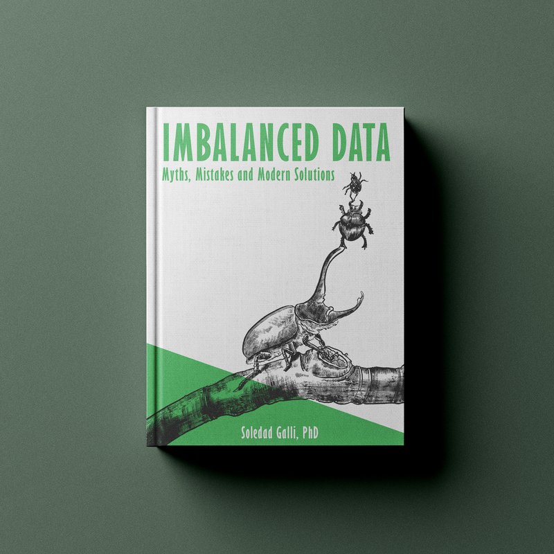
To master probability calibration, check out my book Imbalanced Data: Myths, Mistakes and Modern Solutions.
Why Is Calibration Essential in Machine Learning?
In machine learning, probability calibration is the process of adjusting a model’s predictions so that they match the actual likelihood of events. For example, when a model predicts a 30% chance of rain, it should rain on about 30% of those days.
Let’s take a look at why calibration is important in data science projects.
Reliable Probability Estimates
Many classifiers rank observations well but return probabilities that are too extreme or too timid. Using those outputs directly as probabilities can lead to poor decisions.
For example, consider a model that predicts whether a patient has tuberculosis (TB) from lung CT scans. If the model is overconfident and predicts an 80% chance of TB when the real chance is 50%, the doctor may recommend aggressive treatment, causing unnecessary stress and medical costs.
Calibration and Imbalanced Data
A common belief is that models trained on imbalanced datasets return biased probabilities. In fact, a well-calibrated model trained on data with 5% fraud should predict low probabilities of fraud for most transactions, because fraud is rare.
What breaks calibration is changing the class balance during training, with resampling methods like SMOTE or with class weights. These make the model overestimate the probability of the minority class, and we then need Platt scaling or isotonic regression to bring the probabilities back in line.
The best approach is to avoid distorting the probabilities in the first place, as we discuss in our article on machine learning with imbalanced data.
Interpretability and Trust
When the model’s outputs represent the actual likelihood of events, stakeholders can understand and trust them. This is crucial in highly regulated industries like finance and healthcare.
Decisions Based on Probabilities
Calibration does not change how well a model ranks observations, so metrics like the ROC-AUC stay the same. It matters whenever we use the probabilities themselves: to estimate risk, to calculate expected costs, to compare models with probability-based metrics like the Brier score or the log loss, or to choose a decision threshold.
What Is Platt Scaling?
Platt scaling is a probability calibration technique that trains a logistic regression with the classifier’s scores as input and the true class as target, to learn how to turn the scores into probabilities.
John Platt originally proposed it in 1999 to transform the outputs of SVMs into probabilities. An SVM separates the classes with a hyperplane, and its score is the signed distance of each observation to that hyperplane: the farther away, the more confident the prediction.
These distances are not probabilities, so Platt proposed passing them through a sigmoid function. Since then, Platt scaling has been applied to many other classifiers, like random forests, gradient boosting machines and neural networks.
Platt scaling was designed for binary classification, but it can also be used for multiclass problems with the one-vs-rest approach. Scikit-learn’s CalibratedClassifierCV takes care of this automatically, fitting one sigmoid per class and normalizing the probabilities so that they add up to 1.
How Does Platt Scaling Work?
Platt scaling works in three steps:
-
We train the classifier on a training set, and use it to score a separate calibration set. Let’s call the score of each observation \(f(x)\) and its true class \(y\).
-
We fit a logistic regression with the scores \(f(x)\) as the only input and the true labels \(y\) as the target:
\[P(y = 1 \mid x) = \frac{1}{1 + \exp\left(A f(x) + B\right)}\]The parameters \(A\) and \(B\) are learned by maximum likelihood, that is, by minimizing the log loss on the calibration set. \(A\) is usually negative, so that higher scores lead to higher probabilities.
-
We use the fitted sigmoid to transform the scores of any new observation into calibrated probabilities.
The calibration set must be different from the training set. If we fit the sigmoid on the data used to train the classifier, the scores will look more reliable than they are, and the calibration will be biased.
Platt also suggested a small correction to avoid overfitting: instead of using 0 and 1 as targets, the logistic regression uses values slightly above 0 and slightly below 1, which depend on the number of observations in each class. Scikit-learn applies this correction automatically.
Implementing Platt Scaling in Python
Let’s see how to implement Platt scaling in Python with scikit-learn.
Creating the Training, Calibration and Test Sets
We start by importing the libraries:
import numpy as np
import pandas as pd
import matplotlib.pyplot as plt
from sklearn.calibration import CalibratedClassifierCV, CalibrationDisplay
from sklearn.datasets import make_classification
from sklearn.ensemble import RandomForestClassifier
from sklearn.frozen import FrozenEstimator
from sklearn.metrics import brier_score_loss, roc_auc_score
from sklearn.model_selection import train_test_split
For this example, we create a synthetic dataset for binary classification with make_classification, with 50,000 observations and roughly the same number of observations in each class:
X, y = make_classification(
    n_samples=50000,
    n_features=20,
    n_informative=10,
    n_redundant=5,
    class_sep=0.8,
    random_state=42,
)
We need three datasets: one to train the classifier, one to fit Platt scaling, and one to evaluate the result. We split the data into 60% for training, and 20% each for calibration and testing:
X_train, X_tmp, y_train, y_tmp = train_test_split(
    X, y, test_size=0.4, random_state=0)

X_cal, X_test, y_cal, y_test = train_test_split(
    X_tmp, y_tmp, test_size=0.5, random_state=0)
Training a Random Forest and Plotting a Calibration Curve
Next, we train a random forest with 100 trees on the training set, and obtain the probabilities for the test set:
rf = RandomForestClassifier(n_estimators=100, random_state=0, n_jobs=-1)
rf.fit(X_train, y_train)

probs_rf = rf.predict_proba(X_test)[:, 1]
To check whether these probabilities are calibrated, we plot a calibration curve with scikit-learn’s CalibrationDisplay. It sorts the predictions into bins, and for each bin, plots the average predicted probability against the fraction of observations that actually belong to the positive class:
fig, ax = plt.subplots(figsize=(6, 6))
CalibrationDisplay.from_predictions(
    y_test, probs_rf, n_bins=10, name="Random forest", ax=ax,
)
ax.set_title("Calibration curve: random forest")
plt.show()
The previous code returns the following plot:
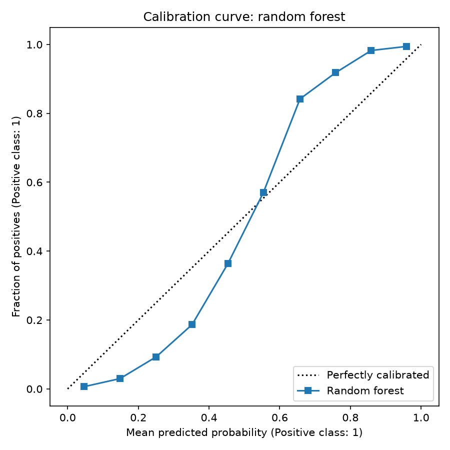
The dotted diagonal shows a perfectly calibrated model, where the predicted probabilities match the fraction of positives. The random forest’s curve has an S shape: when it predicts a probability of about 0.25, only 9% of those observations are positive, and when it predicts about 0.65, 84% of them are.
In other words, the random forest is underconfident: it pushes its predictions toward the middle of the range. This is typical of random forests, because averaging the votes of many trees rarely produces probabilities close to 0 or 1.
Advance your data science and machine learning skills with our comprehensive expert led courses.

Applying Platt Scaling With CalibratedClassifierCV
To apply Platt scaling, we use scikit-learn’s CalibratedClassifierCV with these parameters:
estimator: the classifier to calibrate, the random forest in our example.method: the calibration method,"sigmoid"for Platt scaling or"isotonic"for isotonic regression.cv: how to obtain the data for calibration. We don’t need it here, because we will calibrate a model that is already trained.
Our random forest is already trained, so we wrap it in FrozenEstimator. This tells scikit-learn to use the model as it is, and to only fit the sigmoid, using the calibration set:
platt = CalibratedClassifierCV(FrozenEstimator(rf), method="sigmoid")
platt.fit(X_cal, y_cal)

probs_platt = platt.predict_proba(X_test)[:, 1]
The calibrated probabilities are those of the test set, which neither the random forest nor the sigmoid has seen during training.
Plotting the Calibration Curve After Platt Scaling
Now, let’s plot the calibration curves before and after Platt scaling:
fig, ax = plt.subplots(figsize=(6, 6))
CalibrationDisplay.from_predictions(
    y_test, probs_rf, n_bins=10, name="Random forest", ax=ax,
)
CalibrationDisplay.from_predictions(
    y_test, probs_platt, n_bins=10, name="Random forest + Platt scaling", ax=ax,
)
ax.set_title("Calibration curve after Platt scaling")
plt.show()
In the following plot, we see that after Platt scaling, the calibration curve, in orange, follows the diagonal much more closely:
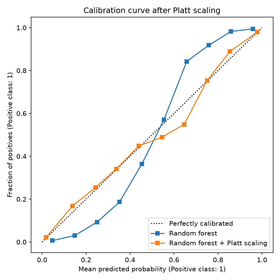
The S-shaped distortion of the random forest is exactly the kind of error a sigmoid can correct, which is why Platt scaling works so well here.
Evaluating Platt Scaling
Let’s compare the probabilities before and after Platt scaling with two metrics. The Brier score measures the mean squared difference between the predicted probabilities and the true outcomes, so lower is better, while the ROC-AUC measures how well the model ranks the observations.
We also calibrate the random forest with isotonic regression, to compare both methods:
iso = CalibratedClassifierCV(FrozenEstimator(rf), method="isotonic")
iso.fit(X_cal, y_cal)
probs_iso = iso.predict_proba(X_test)[:, 1]

pd.DataFrame({
    "Brier score": [
        brier_score_loss(y_test, p) for p in (probs_rf, probs_platt, probs_iso)
    ],
    "ROC-AUC": [
        roc_auc_score(y_test, p) for p in (probs_rf, probs_platt, probs_iso)
    ],
}, index=["Random forest", "Platt scaling", "Isotonic regression"]).round(3)
In the following output, we see the Brier score and ROC-AUC of each model:
                     Brier score  ROC-AUC
Random forest              0.055    0.984
Platt scaling              0.044    0.984
Isotonic regression        0.044    0.983
Platt scaling reduces the Brier score from 0.055 to 0.044, while the ROC-AUC stays the same, because the sigmoid preserves the order of the observations. Isotonic regression reaches the same Brier score, but Platt scaling does it with only two parameters.
When the distortion does not follow a sigmoid shape, for example when the probabilities jump abruptly, isotonic regression usually does a better job. We cover it in our guide to isotonic regression.
Platt Scaling With Cross-validation
If we don’t have enough data for a separate calibration set, we can let CalibratedClassifierCV handle the split with cross-validation. In this case, we pass an untrained classifier, and fit it on the combined training and calibration data:
X_train_full = np.vstack([X_train, X_cal])
y_train_full = np.concatenate([y_train, y_cal])

platt_cv = CalibratedClassifierCV(
    RandomForestClassifier(n_estimators=100, random_state=0, n_jobs=-1),
    method="sigmoid",
    cv=5,
)
platt_cv.fit(X_train_full, y_train_full)

probs_cv = platt_cv.predict_proba(X_test)[:, 1]
print(f"Brier score: {brier_score_loss(y_test, probs_cv):.3f}")
With cv=5, scikit-learn trains a random forest on 4 folds and fits the sigmoid on the remaining fold, 5 times, and averages the probabilities of the 5 calibrated models. In the following output, we see that the result is similar to that of the dedicated calibration set:
Brier score: 0.043
Other Calibration Methods
In addition to Platt scaling, data scientists commonly use isotonic regression, beta calibration and temperature scaling. The following table compares them:
| Method | Type | Parameters | Overfitting risk | Best for |
|---|---|---|---|---|
| Platt scaling | Parametric, sigmoid | 2 | Low | Sigmoid-shaped distortions, SVMs, small calibration sets |
| Isotonic regression | Non-parametric, step function | One per step | High on small datasets | Any monotonic distortion, large calibration sets |
| Beta calibration | Parametric, beta family | 3 | Low | Distortions that a sigmoid cannot fit |
| Temperature scaling | Parametric | 1 | Very low | Multiclass neural networks |
Isotonic regression is the most flexible, and it is fast to train, but it needs more data to avoid overfitting. Temperature scaling divides the outputs of a neural network by a single value before the softmax, which makes it simple and popular in deep learning.
Advantages of Platt Scaling
- It works well with small calibration sets, because it has only two parameters and is hard to overfit.
- It is fast to train and to apply.
- It is easy to interpret, since it is a logistic regression with a single input.
- It preserves the ranking of the observations, so metrics like the ROC-AUC don’t change.
Limitations of Platt Scaling
- It can only correct sigmoid-shaped distortions. If the miscalibration has a different shape, isotonic regression or beta calibration usually work better.
- It was designed for binary classification. For multiclass problems, it relies on the one-vs-rest approach, while temperature scaling handles all classes at once.
To learn about other calibration methods, check out my book Imbalanced Data: Myths, Mistakes and Modern Solutions.
Conclusion
Platt scaling is a simple and effective calibration technique for binary classification tasks like fraud detection, disease prediction or sports forecasting. It turns raw scores, like those of SVMs, or miscalibrated probabilities, like those of random forests, into probabilities we can trust.
Remember to fit it on data the classifier has not seen, and to check the calibration curve afterward. Calibrated probabilities help data scientists estimate risk and make better decisions.
Additional Resources
- Niculescu-Mizil and Caruana. 2005. Predicting Good Probabilities With Supervised Learning. Proceedings of the 22nd International Conference on Machine Learning.
- Scikit-learn documentation: CalibratedClassifierCV.
