ADASYN: Adaptive Synthetic Sampling for Imbalanced Datasets

ADASYN is an oversampling method that creates synthetic examples of the minority class to balance an imbalanced dataset. It was proposed as an improvement over SMOTE, generating more synthetic data where the minority class is hardest to learn.

Here is the catch. ADASYN leaves the model’s ability to tell the classes apart unchanged. All it does is shift the decision boundary, so that at the default threshold of 0.5 the model flags more observations as the minority class.

We can get the same effect by training the model on the original data and lowering the classification threshold, without generating a single synthetic example. In this article, we’ll show this with Python code.

We’ll cover:

• What ADASYN is and how the algorithm works
• How ADASYN compares with SMOTE
• How to apply ADASYN in Python with imbalanced-learn
• Why moving the threshold gives the same result
• The limitations of ADASYN

For a modern take on how to work with imbalanced data, check out my book Imbalanced Data: Myths, Mistakes and Modern Solutions.

What Is ADASYN?

ADASYN, short for Adaptive Synthetic Sampling, was proposed by Haibo He, Yang Bai, Edwardo A. Garcia and Shutao Li in their 2008 article “ADASYN: Adaptive Synthetic Sampling Approach for Imbalanced Learning”. It is an oversampling technique designed to address class imbalance.

ADASYN is an extension of SMOTE, the Synthetic Minority Over-sampling Technique. SMOTE uses every minority class example as a template for new synthetic data with the same probability.

ADASYN, instead, creates more synthetic examples around the minority observations that are surrounded by the majority class, which are the hardest to classify. The idea is to push the decision boundary further toward those difficult examples.

How Does ADASYN Work?

ADASYN relies on k-nearest neighbors to find out how difficult each minority example is to learn, and then decides how many synthetic examples to create around each one. Let’s go through the algorithm step by step.

Step 1: Calculate the Number of Synthetic Examples

ADASYN starts by measuring the degree of imbalance, the ratio between the number of minority and majority examples. If the imbalance is larger than a tolerated level, it calculates the total number of synthetic examples to generate:

\[G = (m_l - m_s) \times \beta\]

Here, \(m_l\) and \(m_s\) are the number of majority and minority examples, and \(\beta\) is a value between 0 and 1. With \(\beta = 1\), which is the default in imbalanced-learn, the resampled dataset ends up fully balanced.

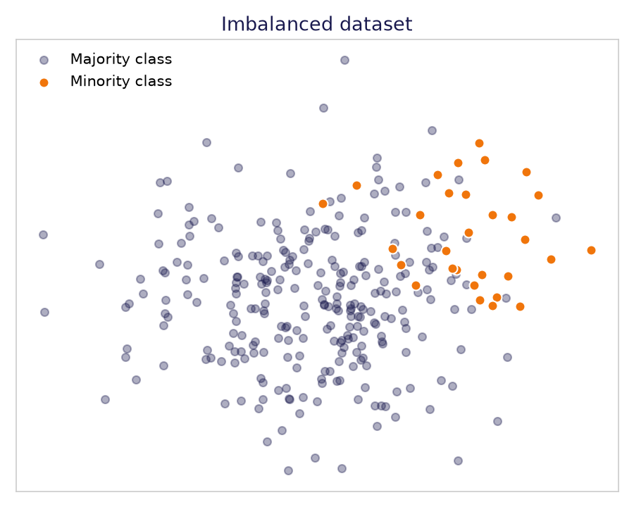
The following image shows an imbalanced dataset with two classes, which we’ll use to illustrate the remaining steps:

Step 2: Identify the Hard-to-Learn Minority Examples

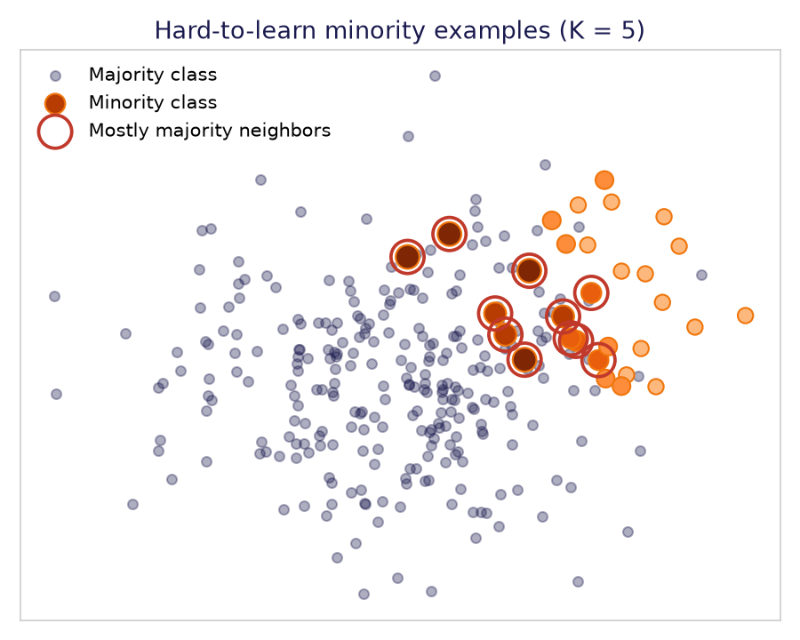
For each minority example \(x_i\), ADASYN finds its K nearest neighbors in the whole dataset and counts how many of them belong to the majority class, \(\Delta_i\). The ratio \(r_i = \Delta_i / K\) tells us how hard the example is to learn.

A minority example surrounded by other minority examples has a ratio of 0, and one surrounded only by majority examples has a ratio of 1. In the following image, the darker and larger the dot, the higher the ratio, and the circled examples have mostly majority class neighbors:

Step 3: Compute the Sampling Distribution

ADASYN normalizes the ratios so that they add up to 1, and then multiplies them by G to obtain the number of synthetic examples to create around each minority example:

\[\hat{r}_i = \frac{r_i}{\sum_j r_j}, \qquad g_i = \hat{r}_i \times G\]

Examples with more majority class neighbors get more synthetic data. Examples surrounded only by the minority class get none.

Step 4: Generate the Synthetic Examples

For each minority example \(x_i\), ADASYN creates \(g_i\) synthetic examples. Each time, it picks one of the nearest neighbors of \(x_i\) from the minority class, \(x_{zi}\), and interpolates between the two:

\[x_{new} = x_i + \lambda \, (x_{zi} - x_i)\]

where \(\lambda\) is a random number between 0 and 1. The new example lies on the line between \(x_i\) and its neighbor, as we see in the following image:

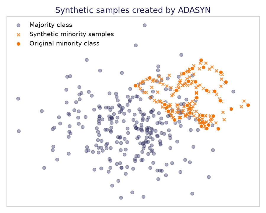
Notice how many synthetic examples land in the region where the two classes overlap, right among the majority class. That is ADASYN working as designed, and it is also the source of its problems, as we’ll see later.

ADASYN vs SMOTE

ADASYN and SMOTE create synthetic data in the same way, by interpolating between a minority example and one of its minority neighbors. They differ in how they choose which examples to use as templates:

• SMOTE picks every minority example with the same probability, so synthetic data spreads across the whole minority class.
• ADASYN picks minority examples in proportion to the number of majority class neighbors they have, so synthetic data concentrates where the classes overlap.

As a result, ADASYN pushes the decision boundary further into the majority class than SMOTE. Neither method gives the model new information to separate the classes, because the synthetic examples are combinations of the data we already have.

Unsure whether SMOTE or ADASYN are the right methods for your project? Read my free booklet “7 Takes on Working with Imbalanced Data”, where I discuss 3 recent articles that change the conversation around resampling.

ADASYN in Python With Imbalanced-learn

Let’s see ADASYN in action. We’ll use the thyroid sick dataset from imbalanced-learn, where the goal is to predict whether a patient is sick.

Loading the Imbalanced Dataset

Let’s import the libraries:

import numpy as np
import pandas as pd
from imblearn.datasets import fetch_datasets
from imblearn.over_sampling import ADASYN
from sklearn.ensemble import RandomForestClassifier
from sklearn.metrics import precision_score, recall_score, roc_auc_score
from sklearn.model_selection import TunedThresholdClassifierCV, train_test_split

Now, we load the dataset. In the original data, the target takes the value 1 for sick patients and -1 for healthy ones, so we convert it to 1 and 0:

data = fetch_datasets(filter_data=("thyroid_sick",))["thyroid_sick"]
X = data.data
y = (data.target == 1).astype(int)

print("Class counts:", np.bincount(y))

The output shows the number of healthy patients, class 0, and sick patients, class 1:

Class counts: [3541  231]

Only 231 of the 3,772 patients are sick, about 6% of the dataset. Next, we split the data into a training set and a test set, keeping the class proportions in both with stratify=y:

X_train, X_test, y_train, y_test = train_test_split(
    X, y, test_size=0.3, random_state=42, stratify=y,
)

print("Train:", np.bincount(y_train))
print("Test: ", np.bincount(y_test))

In the following output, we see that both sets keep the original proportion of sick patients:

Train: [2478  162]
Test:  [1063   69]

Training a Baseline Model on the Imbalanced Data

We’ll evaluate several models in the same way, so let’s write a small function that returns the precision and recall at a given threshold, and the ROC-AUC:

def evaluate(model, X_test, y_test, threshold=0.5):
    proba = model.predict_proba(X_test)[:, 1]
    pred = (proba >= threshold).astype(int)
    print(f"Precision: {precision_score(y_test, pred):.3f}")
    print(f"Recall:    {recall_score(y_test, pred):.3f}")
    print(f"ROC-AUC:   {roc_auc_score(y_test, proba):.3f}")

Precision tells us how many of the patients flagged as sick are actually sick, and recall how many of the sick patients the model finds. You can learn more about these metrics in our article on the confusion matrix, precision and recall.

Now, we train a random forest on the original, imbalanced training set:

base_model = RandomForestClassifier(random_state=42)
base_model.fit(X_train, y_train)

evaluate(base_model, X_test, y_test)

These are the precision, recall and ROC-AUC of the baseline model on the test set:

Precision: 0.937
Recall:    0.855
ROC-AUC:   0.998

At the default threshold of 0.5, the model finds 85.5% of the sick patients, so it misses about 14% of them. In healthcare, missing a sick patient is usually worse than a false alarm, so we’d like a higher recall.

Oversampling the Training Set With ADASYN

Let’s apply ADASYN to the training set. We never resample the test set, because it must reflect the real class distribution:

adasyn = ADASYN(random_state=42)
X_res, y_res = adasyn.fit_resample(X_train, y_train)

print("After ADASYN:", np.bincount(y_res))

In the following output, we see the number of observations in each class after ADASYN:

After ADASYN: [2478 2512]

The resampled training set is now roughly balanced. ADASYN produces approximately, but not exactly, the same number of examples in each class, because it rounds the number of synthetic examples per minority observation.

Training a Model on the ADASYN Data

We train a second random forest on the resampled data, and evaluate it on the same test set:

adasyn_model = RandomForestClassifier(random_state=42)
adasyn_model.fit(X_res, y_res)

evaluate(adasyn_model, X_test, y_test)

And these are the metrics of the model trained on the ADASYN data:

Precision: 0.875
Recall:    0.913
ROC-AUC:   0.998

The recall went up from 0.855 to 0.913, and the precision went down from 0.937 to 0.875. The model now flags more patients as sick, catching more of the sick ones at the cost of more false alarms.

Now look at the ROC-AUC, which stayed at 0.998. The ROC-AUC measures how well the model ranks sick patients above healthy ones across all thresholds, so ADASYN left the model’s ability to separate the classes untouched and only moved the point where the model says “sick.”

Moving the Threshold Instead of Oversampling

If ADASYN only moves the decision boundary, we should be able to get the same result by moving the threshold of the model trained on the original data. Let’s check.

ADASYN Gives the Same Trade-off as a Lower Threshold

We take the probabilities of the baseline model, the one trained without ADASYN, and calculate precision and recall at several thresholds:

proba_base = base_model.predict_proba(X_test)[:, 1]

rows = []
for t in [0.5, 0.45, 0.4, 0.35, 0.3]:
    pred = (proba_base >= t).astype(int)
    rows.append({
        "threshold": t,
        "precision": precision_score(y_test, pred),
        "recall": recall_score(y_test, pred),
    })

print(pd.DataFrame(rows).round(3).to_string(index=False))

In the following table, we see the precision and recall of the baseline model at each threshold:

 threshold  precision  recall
      0.50      0.937   0.855
      0.45      0.897   0.884
      0.40      0.887   0.913
      0.35      0.833   0.942
      0.30      0.786   0.957

At a threshold of 0.4, the model trained on the original data reaches exactly the same recall as the ADASYN model, 0.913, with a slightly higher precision, 0.887 instead of 0.875. We got the ADASYN result without creating any synthetic data.

The table also shows the full precision-recall trade-off. By moving the threshold, we can choose any balance between finding sick patients and raising false alarms, which is much more flexible than resampling. We discuss this trade-off in depth in our article on precision-recall curves.

Tuning the Threshold With TunedThresholdClassifierCV

In the previous table, we looked at the test set to compare the two approaches. To choose a threshold in practice, we must use the training data only, otherwise our evaluation will be too optimistic.

Scikit-learn’s TunedThresholdClassifierCV does this for us. It finds the threshold that maximizes a metric with cross-validation on the training set, and then applies it when we call predict():

tuned_model = TunedThresholdClassifierCV(
    estimator=RandomForestClassifier(random_state=42),
    scoring="f1",
    cv=5,
)
tuned_model.fit(X_train, y_train)

print(f"Best threshold: {tuned_model.best_threshold_:.2f}")

pred = tuned_model.predict(X_test)
print(f"Precision: {precision_score(y_test, pred):.3f}")
print(f"Recall:    {recall_score(y_test, pred):.3f}")

The output shows the threshold found with cross-validation, followed by the precision and recall on the test set:

Best threshold: 0.32
Precision: 0.793
Recall:    0.942

The tuned model finds 94% of the sick patients, more than the ADASYN model, at a lower precision. Here we maximized the F1 score, but we can pass any metric to scoring, including a custom one that reflects the real cost of each error, which leads to cost-sensitive decisions.

ADASYN Also Distorts the Predicted Probabilities

There is one more reason to prefer moving the threshold. When we train on balanced data, the model learns that half of the observations are positive, so it overestimates the probability of the minority class:

proba_adasyn = adasyn_model.predict_proba(X_test)[:, 1]

print(f"Fraction of sick patients:       {y_test.mean():.3f}")
print(f"Mean probability, original data: {proba_base.mean():.3f}")
print(f"Mean probability, ADASYN data:   {proba_adasyn.mean():.3f}")

In the following output, we compare the real fraction of sick patients with the average probability predicted by each model:

Fraction of sick patients:       0.061
Mean probability, original data: 0.067
Mean probability, ADASYN data:   0.078

The model trained on the original data predicts, on average, a probability close to the real fraction of sick patients. The ADASYN model overestimates it, and the effect is usually much stronger with weaker models.

If we need probabilities we can trust, for example to estimate risk, resampling forces us to recalibrate the model afterward. We explain why in our article on probability calibration.

Limitations of ADASYN

To sum up, these are the main drawbacks of ADASYN:

• It does not improve discrimination: synthetic examples are interpolations of existing data, so the model learns nothing new about how to separate the classes. As we saw, the ROC-AUC stays the same.
• It amplifies noise: a minority example surrounded only by majority examples gets the highest weight, even when it is an outlier or a labeling error. ADASYN then fills the majority class region with synthetic data based on it.
• It creates unrealistic data: interpolating between examples can create combinations of feature values that don’t exist in reality, especially with categorical or discrete variables.
• It distorts probabilities: models trained on resampled data overestimate the probability of the minority class.
• It adds computation: ADASYN needs nearest neighbor searches, which become slow with large and high-dimensional datasets, and it makes the training set bigger.

Conclusion

ADASYN was introduced to deal with imbalanced datasets by focusing synthetic data on the hardest-to-learn minority examples. In practice, it shifts the decision boundary toward the minority class, which is the same trade-off between precision and recall that we get by lowering the classification threshold.

So, our recommendation is to avoid synthetic data generation. Train a strong model, like gradient boosting or a random forest, on the original data.

This is simpler and faster, it keeps the predicted probabilities meaningful, and it lets you move along the whole precision-recall trade-off instead of being stuck with the point that resampling gives you. For more on this, check out our article on machine learning with imbalanced data.

Additional Resources

• The original ADASYN paper, published at the 2008 IEEE International Joint Conference on Neural Networks: ADASYN: Adaptive Synthetic Sampling Approach for Imbalanced Learning.

To learn more about working with imbalanced data, the techniques used in industry, and much more, check out my book Imbalanced Data: Myths, Mistakes and Modern Solutions.