Should You Use Imbalanced-Learn in 2025?

Imbalanced-learn is a Python open-source library that supports methods that have longed been proposed as effective to tackle alleged poor performance of machine learning models trained using imbalanced datasets.

Among the methods supported by imbalanced-learn, we find oversampling and data generating techniques like SMOTE; undersampling and data cleaning methods, like Edited Nearest Neighbors and Condensed Nearest Neighbors; and bagging and boosting algorithms specifically designed to perform better with imbalanced datasets, like EasyEnsemble and RusBoost.

Imbalanced-learn also supports specific model evaluation metrics designed to, in theory, better determine a machine learning model‘s performance that was trained on imbalanced data.

But, are these methods and tools really effective to tackle imbalanced data? That’s what we’ll discuss throughout this article.

Get your free copy of my “7 Takes on Working with Imbalanced Data“, where I discuss 3 recent articles that change the conversation around resampling.

The short answer, up front: undersampling, oversampling, SMOTE, and cost-sensitive learning don’t make a model better at discriminating between classes. What they do is shift the decision boundary so that, at the default classification threshold of 0.5, we make more cost-sensitive decisions — we correctly flag a larger proportion of the minority class, which is usually the class we care about most. You can get that exact same effect by training on the original, unmodified data and adjusting the classification threshold afterward, without touching imbalanced-learn at all. The rest of this article walks through the evidence for that claim.

Imbalanced datasets – what are they?

Imbalanced datasets—datasets where one class significantly outnumbers others—are a common occurrence in real-world applications, such as fraud detection or disease diagnosis, among others.

When classes are imbalanced, machine learning algorithms are said to favor the majority class, leading to poor predictions for the minority class. That is certainly true for the so called “weak learners”, like decision trees and support vector machines. Strong classifiers have been shown to be effective at predicting the minority class in spite of the imbalance (read on).

Methods to tackle class imbalance

To address this “class imbalance problem”, various methods have been described and later on implemented in the Python library Imbalanced-Learn. These methods are said to enhance model performance and ensure that minority classes are accurately represented in predictions.

Among the methods designed to tackle the alleged classification problems said to occur when using imbalanced datasets in machine learning, we find:

• Oversampling and data augmentation methods, like random oversampling and SMOTE and its variants.
• Undersampling and data cleaning techniques, like random undersampling, Edited Nearest Neighbors and the Neighborhood Cleaning Rule.
• Bagging and Boosting algorithms that include under- or oversampling while generating the bootstrapped datasets that are used to train each tree in the ensemble, like EasyEnsemble.

But… do these methods really work?

The hype of SMOTE

SMOTE is a data generating method, said to create datapoints that look like those from the minority class. By adding more minority class-look like examples to the dataset, we remove the imbalance and hence, shift the decision boundary toward the minority class — or so the story goes.

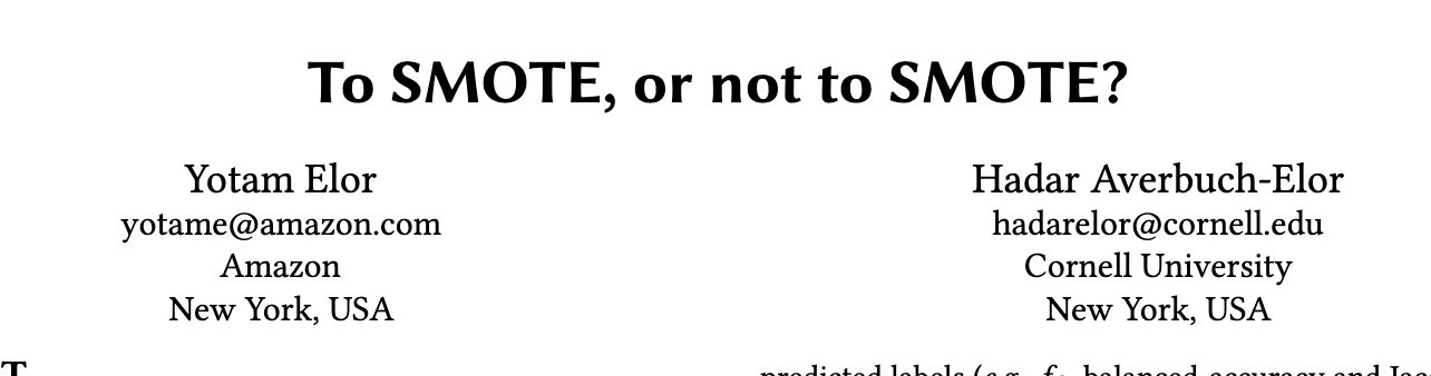
In 2022, a scientific article came out, making a systematic comparison of the performance of various machine learning models, including weak and strong learners, trained to classify various imbalanced datasets, with and without the use of random oversampling and SMOTE.

Weak learners included decision trees, support vector machines and adaboost, and strong learners included xgboost and catboost.

To evaluate model performance they used threshold dependent metrics, like precision and recall, and threshold independent metrics like the ROC-AUC.

For the threshold dependent metrics, they compared the model performance returned when the metric was calculated using the “classical” 0.5 probability threshold, or a more suitable threshold for imbalanced classes, that will typically be somewhere below 0.5.

What they saw, is that random oversampling and SMOTE did indeed show an increase in model performance WHEN, the threshold dependent metrics were calculated using a probability threshold of 0.5. HOWEVER, and this is the important bit, the same effect could be obtained when calculating the metric using a tuned threshold, WITHOUT oversampling or SMOTE.

What does this mean? that the whole SMOTE hype was based on metrics that were calculated wrongly, by not adjusting the probability threshold, something that is common practice in data science, when working with imbalanced classes.

In fact, if you want to see these evidence in action, check out Guillaume Lamaitre’s (one of the imbalanced-learn developers) talk, where he discusses this issue and demonstrates it with Python code using scikit-learn.

In fact, glemaitre goes on to discourage the use of SMOTE, ADASYN and TOMEK Links (a cleaning method), and instead tune the probability threshold when working with imbalanced datasets.

So, does oversampling not work?

The authors of the 2024 article “To SMOTE or not to SMOTE”, concluded that if we use strong classifiers like xgboost, then oversampling or SMOTE do not really help improve the model’s performance.

The identified, however, a few scenarios where oversampling and SMOTE might be useful, and they are:

• SMOTE-like methods could improve the performance of “weak” learners like multilayer perceptrons, decision trees, support vector machines, and, interestingly, lightGBMs.
• SMOTE-like methods could improve the performance of models that do not return a probability as output, and hence, we can’t optimize the threshold to calculate the threshold dependent metrics.

However, on the later, they mentioned that random oversampling returned similar results to SMOTE, and is yet a simpler technique, so random oversampling is recommended over SMOTE.

So, should you use imbalanced-learn in 2024?

Well, for oversampling methods, only if you are training weak learners. But the recommendation is, of course, to use strong classifiers like xgboost and tune the probability threshold.

Undersampling methods for imbalanced datasets

Undersampling methods reduce the number of samples of the majority class. There are various methods, typically divided into cleaning or fixed undersampling.

Fixed undersampling methods reduce the number of samples up to a certain extent, defined by the user. For example, they reduce the number of observations until we have equal number of samples of the majority and minority class. The classical method is random undersampling, while the instance hardness threshold is another fixed undersampling technique.

Cleaning undersampling methods, instead, remove “problematic” observations. Problematic observations are usually those that are hard to classify, for one reason or another. For example, they’d remove observations from the majority class if they are surrounded mostly by observations of the minority class. All cleaning methods involve the use of k-nearest neighbors (knn) to find those observations to remove, and hence “clean” the data.

Unfortunately, there is not a thorough study comparing the performance of the various undersampling methods across datasets. So whether these methods are effective in the light of strong classifiers like xgboost, remains a question.

I made a comparison of various fixed and cleaning undersampling methods, including Tomek links and nearmiss, across publicly available datasets in this github repo. I saw that random undersampling and the instance hardness threshold do improve model performance in SOME datasets. But in most datasets, undersampling methods did not improve the performance of random forests.

To master the use of fixed and cleaning undersampling methods, check out my book Machine Learning with Imbalanced Data.

So, does undersampling work?

The advice for undersampling is probably similar to that for oversampling. These methods may improve model performance when training weak classifiers, like logistic regression or decision trees. I also saw some benefits for random forests for certain datasets. But, although this still needs to be tested, they may not add a lot of value when using strong classifiers like xgboost.

Having said this, cleaning methods based on knn take long to run and are not scalable. So there is an additional constraint: if datasets are big, computation time might get quite high. And life gets on, you know…

Bagging and Boosting algorithms for imbalanced datasets

Throughout the years, various Bagging and Boosting methods that add a step of under- or oversampling while creating the bootstrapped datasets to train the model have been described. Do we really need them?

Again, unfortunately, there has been no systematic comparison that evaluates and compares the performance of these models to xgboost or catboost. Hence, it is hard to say, if adding the complexity of undersampling or oversampling during the induction of the model, is worth the effort (and computation cost).

Imbalanced learn supports the following specially designed bagging and boosting algorithms:

• EasyEnsemble
• RusBoost
• Balanced Random Forests
• Balanced classifiers (it balances the data to bag any classifier)

In this repo, I compared the performance of EasyEnsemble, RusBoost and Balanced Random Forests across datasets, to that of normal Random Forests, Adaboost and Bagged Adaboost. This is what I found:

• In 7 datasets, adaboost clearly outperformed random forests, but random forests never outperformed adaboost.

We expected that, because boosting is, in general, a better model than just bagging.

• Balanced random forests and EasyEnsemble outperformed adaboost in 8 and 10 datasets, respectively.

These 2 models are quite promising, and the good news is, that they are relatively fast to train.

• Bagging of adaboost and RusBoost showed good performance overall, but it is less clear if their performance is significantly superior to that of adaboost alone.

Bagging adaboost and RusBoost are quite costly in computational terms, so, unless we have access to good computing resources, we can stick to balanced random forests and EasyEnsemble.

Again, I did not compare these models to xgboost, so whether these specially designed ensembles outperform strong classifiers remains a question.

So, should we use imbalanced-learn in 2025?

As the latest evidence suggests, the advice when working with imbalanced data goes as follows:

1. Use strong classifiers when possible like xgboost or catboost.
2. Evaluate performance by combining the use of a threshold dependent and a threshold independent metric.
3. For threshold dependent metrics (like precision or recall), optimize the threshold, do not use the default 0.5

After setting this benchmark, if you want to test something else, cost-sensitive learning is the best first approach.

If you still feel that you need to improve model performance, and are, for some reason, using weaker learners, then you can try undersampling or oversampling methods. Keep in mind that simpler solutions like random under- or oversampling tend to give similar results to more complex methods like data generation with SMOTE or cleaning methods that use KNNs, so there is no need to over-complicate things. Start simple, and go from there.

For random under- or oversampling, there is not need to use imbalanced-learn, you can resample your dataset with mainstream libraries like pandas or numpy.

If you are still curious about imbalanced-learn, below I’ll show you how to install and use this library.

To master the use of imbalanced-learn, check out my book Machine Learning with Imbalanced Data.

Imbalanced-Learn: A Python Library for Resampling

Imbalanced-Learn is an open-source Python library specifically designed to handle class imbalance in datasets. Built to work seamlessly with Scikit-learn, Imbalanced-Learn provides an extensive suite of resampling techniques, allowing data scientists to rebalance datasets effectively.

The library includes methods for oversampling, undersampling, and hybrid sampling, making it versatile and well-suited for various ML applications.

The installation of Imbalanced-Learn is straightforward:

pip install imbalanced-learn

Techniques for Balancing Data in Imbalanced-Learn

Imbalanced-Learn offers several techniques for balancing datasets. The three primary methods are oversampling, undersampling, and hybrid sampling. Let’s look at each one of them.

1. Oversampling

Oversampling techniques increase the representation of the minority class by generating synthetic data points or duplicating existing samples. This shifts the decision boundary toward the minority class, so at the default threshold, fewer of its examples get missed.

Random Oversampling: This basic technique randomly duplicates instances of the minority class to balance the dataset. It’s simple to implement but can lead to overfitting, because we are in essence, duplicating data points.

Here’s how to apply random oversampling with imblearn:

import pandas as pd
import matplotlib.pyplot as plt

from sklearn.datasets import make_classification
from imblearn.over_sampling import RandomOverSampler

# Step 1: Create a synthetic imbalanced dataset
X, y = make_classification(
n_samples=500,
n_features=2,
n_informative=2,
n_redundant=0,
n_clusters_per_class=1,
weights=[0.9, 0.1],
flip_y=0,
random_state=42
)

# Step 2: Visualize the original dataset before oversampling
plt.figure(figsize=(12, 5))
plt.subplot(1, 2, 1)
plt.scatter(X[y == 0][:, 0], X[y == 0][:, 1], label="Class 0", alpha=0.5, edgecolor="k")
plt.scatter(X[y == 1][:, 0], X[y == 1][:, 1], label="Class 1", alpha=0.5, edgecolor="k")
plt.title("Original Imbalanced Dataset")
plt.xlabel("Feature 1")
plt.ylabel("Feature 2")
plt.legend()

# Step 3: Apply RandomOverSampler to balance the dataset
oversample = RandomOverSampler(sampling_strategy='minority', random_state=42)
X_over, y_over = oversample.fit_resample(X, y)

# Step 4: Visualize the dataset after oversampling
plt.subplot(1, 2, 2)
plt.scatter(X_over[y_over == 0][:, 0], X_over[y_over == 0][:, 1], label="Class 0", alpha=0.5, edgecolor="k")
plt.scatter(X_over[y_over == 1][:, 0], X_over[y_over == 1][:, 1], label="Class 1", alpha=0.5, edgecolor="k")
plt.title("Dataset After Random Oversampling")
plt.xlabel("Feature 1")
plt.ylabel("Feature 2")
plt.legend()

plt.tight_layout()
plt.show()

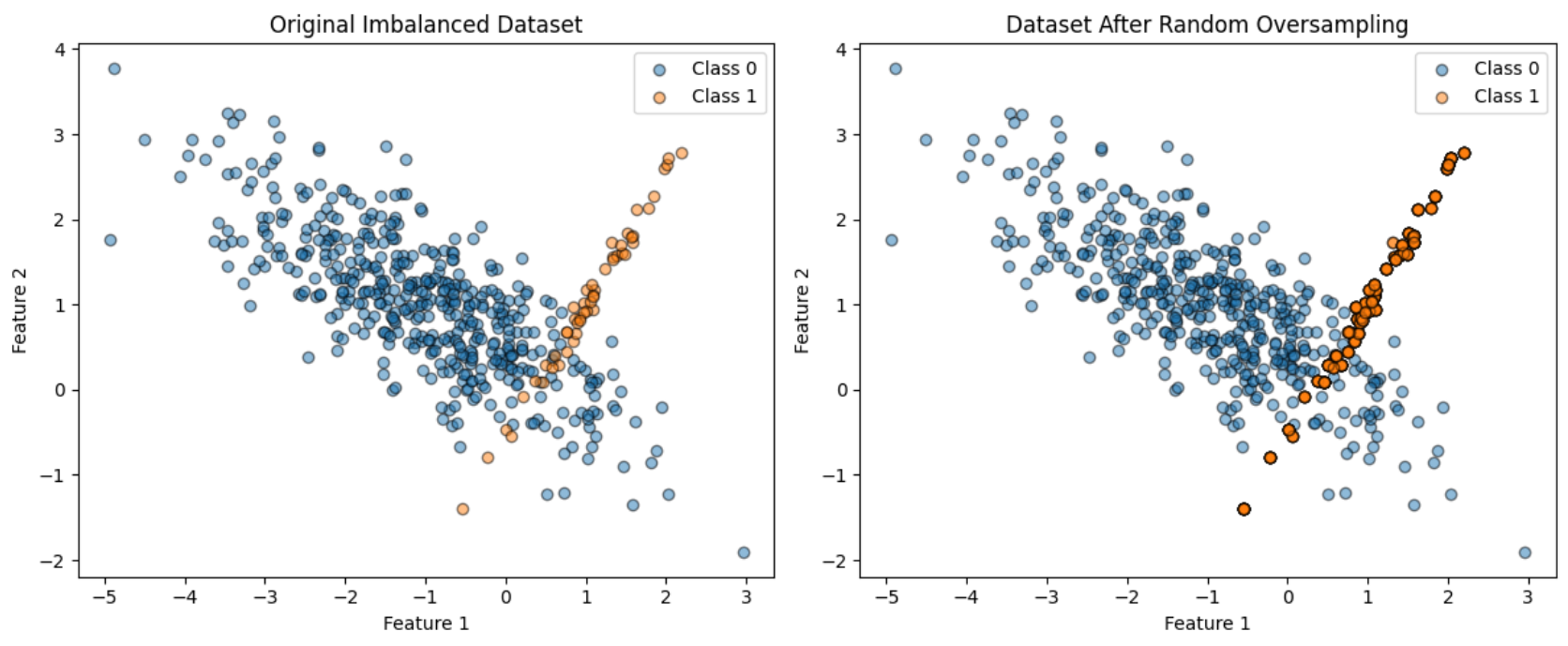
In the following image, we compare the original classes distribution, with the data distribution after applying random oversampling. Note that we see exactly the same data points for the minority class, just in darker orange, due to the overlay of points on themselves:

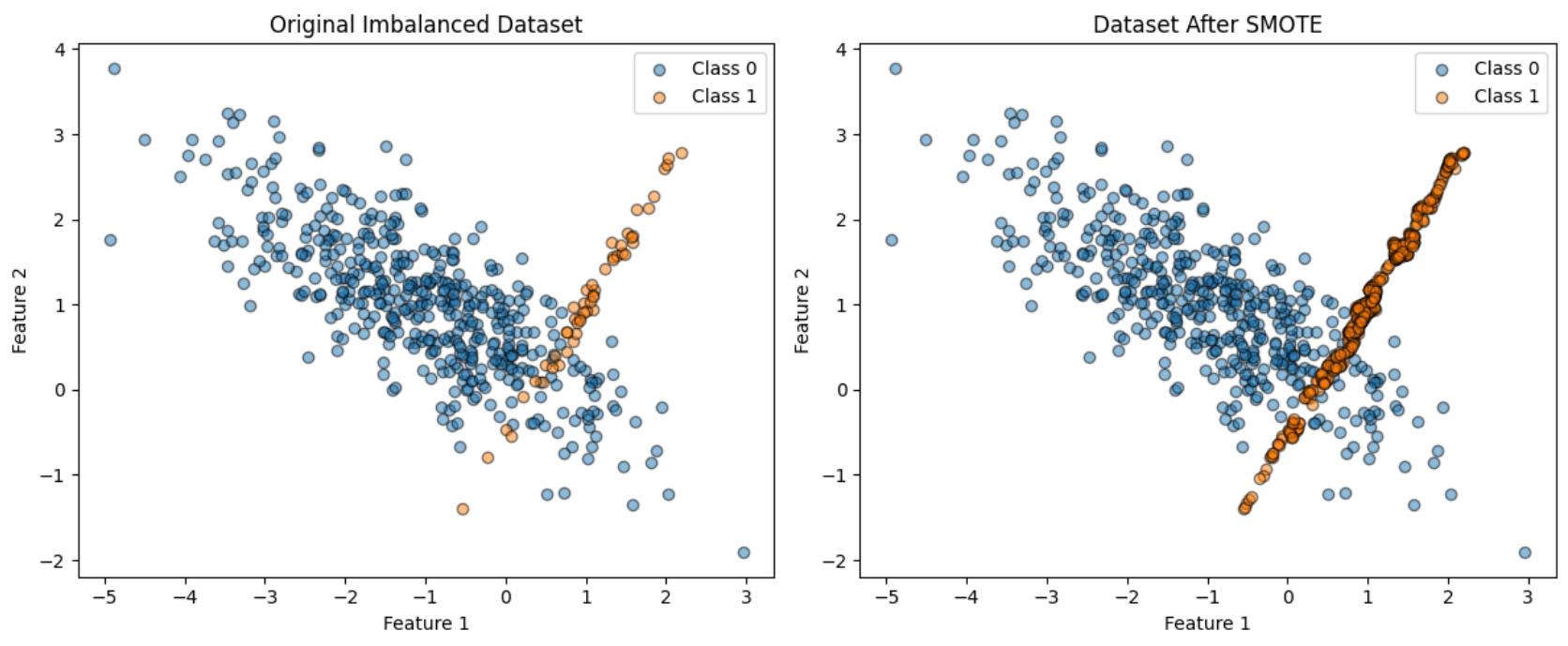
Synthetic Minority Over-sampling Technique (SMOTE): SMOTE generates new data resembling the minority class by interpolating between existing instances of the minority class.

Here’s how to implement it with imblearn:

from imblearn.over_sampling import SMOTE

smote = SMOTE()
X_smote, y_smote = smote.fit_resample(X, y)

plt.figure(figsize=(12, 5))
plt.subplot(1, 2, 1)
plt.scatter(X[y == 0][:, 0], X[y == 0][:, 1], label="Class 0", alpha=0.5, edgecolor="k")
plt.scatter(X[y == 1][:, 0], X[y == 1][:, 1], label="Class 1", alpha=0.5, edgecolor="k")
plt.title("Original Imbalanced Dataset")
plt.xlabel("Feature 1")
plt.ylabel("Feature 2")
plt.legend()

plt.subplot(1, 2, 2)
plt.scatter(X_smote[y_smote == 0][:, 0], X_smote[y_smote == 0][:, 1], label="Class 0", alpha=0.5, edgecolor="k")
plt.scatter(X_smote[y_smote == 1][:, 0], X_smote[y_smote == 1][:, 1], label="Class 1", alpha=0.5, edgecolor="k")
plt.title("Dataset After SMOTE")
plt.xlabel("Feature 1")
plt.ylabel("Feature 2")
plt.legend()

plt.tight_layout()
plt.show()

In the following image, we compare the distribution of the minority class after creating synthetic examples. Note that we are not simply duplicating points, there are newer data examples:

2. Undersampling

Undersampling reduces the size of the majority class, balancing the dataset by removing excess samples. While undersampling can result in data loss, it can be useful when dealing with large majority classes that may lead to computational inefficiencies.

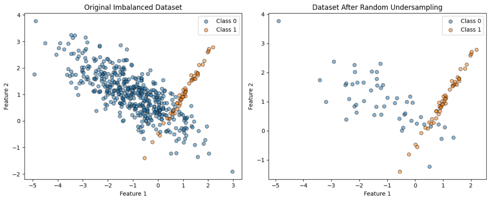
Random Undersampling: This technique randomly removes samples from the majority class to achieve balance. It’s simple but can risk losing valuable information from the majority class.

Here’s how to implement it with imblearn:

from imblearn.under_sampling import RandomUnderSampler

undersample = RandomUnderSampler()
X_under, y_under = undersample.fit_resample(X, y)

plt.figure(figsize=(12, 5))
plt.subplot(1, 2, 1)
plt.scatter(X[y == 0][:, 0], X[y == 0][:, 1], label="Class 0", alpha=0.5, edgecolor="k")
plt.scatter(X[y == 1][:, 0], X[y == 1][:, 1], label="Class 1", alpha=0.5, edgecolor="k")
plt.title("Original Imbalanced Dataset")
plt.xlabel("Feature 1")
plt.ylabel("Feature 2")
plt.legend()

plt.subplot(1, 2, 2)
plt.scatter(X_under[y_under == 0][:, 0], X_under[y_under == 0][:, 1], label="Class 0", alpha=0.5, edgecolor="k")
plt.scatter(X_under[y_under == 1][:, 0], X_under[y_under == 1][:, 1], label="Class 1", alpha=0.5, edgecolor="k")
plt.title("Dataset After Random Undersampling")
plt.xlabel("Feature 1")
plt.ylabel("Feature 2")
plt.legend()

plt.tight_layout()
plt.show()

In the following image, we compare the class distributions before and after undersampling the majority class:

Edited Nearest Neighbours (ENN): ENN is an undersampling method that removes instances in the majority class if their nearest neighbors belong to a different class. This technique shifts the decision boundary by cleaning up majority class samples near it.

Here’s how to implement it with imblearn:

from imblearn.under_sampling import EditedNearestNeighbours

enn = EditedNearestNeighbours()
X_en, y_en = enn.fit_resample(X, y)

plt.figure(figsize=(12, 5))
plt.subplot(1, 2, 1)
plt.scatter(X[y == 0][:, 0], X[y == 0][:, 1], label="Class 0", alpha=0.5, edgecolor="k")
plt.scatter(X[y == 1][:, 0], X[y == 1][:, 1], label="Class 1", alpha=0.5, edgecolor="k")
plt.title("Original Imbalanced Dataset")
plt.xlabel("Feature 1")
plt.ylabel("Feature 2")
plt.legend()


plt.subplot(1, 2, 2)
plt.scatter(X_en[y_en == 0][:, 0], X_en[y_en == 0][:, 1], label="Class 0", alpha=0.5, edgecolor="k")
plt.scatter(X_en[y_en == 1][:, 0], X_en[y_en == 1][:, 1], label="Class 1", alpha=0.5, edgecolor="k")
plt.title("Dataset After ENN")
plt.xlabel("Feature 1")
plt.ylabel("Feature 2")
plt.legend()

plt.tight_layout()
plt.show()

In the following image, we compare the class distributions before and after applying the cleaning method edited nearest neighbor. Note how the method has removed observations from the majority class closed to those of the minority class:

3. Hybrid Sampling

Hybrid methods combine oversampling and undersampling techniques, aiming to balance datasets while avoiding overfitting or data loss. These methods are ideal for datasets that require a balanced approach to ensure both classes are represented adequately without excessive repetition or removal.

The python implementation is similar to those of under- or oversampling techniques: we just import the resampler and apply it with fit_resample.

Evaluation Metrics for Imbalanced Data

After resampling, it’s essential to assess the effectiveness of the approach. Standard evaluation metrics like accuracy can be misleading for imbalanced datasets, so alternative metrics like precision, recall, F1-score, and the Area Under the Receiver Operating Characteristic Curve (AUC-ROC) are recommended.

• Precision: Measures the proportion of true positive predictions among all positive predictions.
• Recall: Indicates the model’s ability to capture all positive instances.
• F1-Score: The harmonic mean of precision and recall, balancing both metrics to provide a more reliable evaluation for imbalanced data.
• ROC-AUC: The area under the ROC curve, which provides insight into the model’s sensitivity across different thresholds.

Comparing these metrics before and after resampling allows for a clear understanding of how the decision boundary shifted at the default threshold — remember, the same shift can usually be achieved by tuning the threshold on the model trained on the original data.

Integrating Imbalanced-Learn with Scikit-Learn and Beyond

One of Imbalanced-Learn’s key strengths is its integration with Scikit-learn. This compatibility allows users to incorporate Imbalanced-Learn’s resampling methods into Scikit-learn pipelines, seamlessly merging data preprocessing, feature selection, and model training steps.

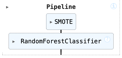
For example, it’s possible to integrate SMOTE within a pipeline to automatically balance classes during the preprocessing stage:

from imblearn.pipeline import Pipeline
from sklearn.ensemble import RandomForestClassifier

pipeline = Pipeline([
   ('smote', SMOTE()),
   ('classifier', RandomForestClassifier())
])

pipeline.fit(X, y)

Below, the evidence that the pipeline worked ;)

Conclusion

Imbalanced-Learn was a great initiative that aimed to democratize and make easily accessible methods to tackle imbalanced datasets, as soon as these methods were described.

Later on, stronger classifiers like xgboost came to the field and more thorough comparisons of the effectiveness of these methods were made, which resulted in data that suggests that over- and under-sampling may, more often than not, not be the one stop solution for imbalanced datasets.

Still, there are some cases where these techniques can add value, and for that, imbalanced-learn can still be valuable, because it provides a framework that allows you to easily integrate these methods with the Python tools that you are used to work with.

If you want to learn more about working with imbalanced datasets, check out my book”: Machine learning with Imbalanced Data.