Probability Calibration in Machine Learning: Enhancing Model Usability

In data science and machine learning, the accuracy of a classifier’s predictions is crucial. Yet, another, often overlooked aspect, is whether the probability estimates returned by the model accurately reflect the likelihood of occurrence of the event. If they don’t, we can correct this through probability calibration.

In this article, we’ll explore probability calibration, why it matters, and how to implement it in Python using scikit-learn.

Master probability calibration with our book Machine Learning with Imbalanced Data – in-depth explanations, practical Python implementations, all calibration methods covered.

What is a Calibrated Probability?

A calibrated probability is a probability estimate from a machine learning model that accurately reflects the true likelihood of an event occurring. In other words, if a well-calibrated classification model predicts a 70% chance of an event happening across multiple instances, we expect the event to occur in about 70% of those cases.

For example, if a calibrated weather model predicts a 30% chance of rain for 100 different days, we would expect it to rain on about 30 of those days. Similarly, in a binary classification task, if a calibrated model assigns a probability of 0.8 to the positive class for 100 samples, approximately 80 of those samples should actually belong to the positive class.

In summary, the output from a classifier with calibrated probability should match the true probability distribution.

Some models, like logistic regression, typically output well-calibrated probabilities for classification tasks right out of the box. However, many other popular algorithms, including random forests and support vector machines (SVMs), often produce uncalibrated probabilities that may not accurately reflect the true likelihood of the predicted outcomes.

Probability Calibration originated in meteorology to assess the reliability of weather forecasts. Subsequently, the machine learning community adopted it to enhance the accuracy of probabilistic predictions in a wide range of applications.

What affects the Calibration of a Probability?

Several factors influence how well a model’s predicted probabilities align with real-world outcomes:

• Model Type: Some algorithms (e.g., logistic regression) naturally produce well-calibrated probabilities, while others (e.g., random forests, SVMs) often require calibration.
• Model Complexity: Overly complex models might overfit, leading to overconfident and poorly calibrated predictions.
• Regularization: Over-regularization can cause under-confident predictions, while under-regularization may lead to over-confidence.
• Data Characteristics:
  • Imbalanced datasets can lead to biased probability estimates.
  • Limited data may result in less reliable calibration.
• Resampling: Undersampling, oversampling, and SMOTE don’t make a model better at discriminating between classes — they shift its decision boundary so more of the minority class gets flagged at the default 0.5 threshold, the same trade-off you’d get by tuning the threshold on the original data instead. That shift is exactly what distorts the probability estimates:
  • Oversampling may inflate minority class probabilities.
  • Undersampling might underestimate majority class probabilities.
• Cost-Sensitive Learning: When different misclassification costs are assigned to different classes, it can skew probability estimates. The model adjusts its decision boundary during training to minimize overall cost — the same effect you could get by adjusting the threshold on a model trained without cost weighting — which can lead to uncalibrated probabilities.

Understanding these influences is crucial for developing models that provide reliable probability estimates in applications where prediction confidence is as important as overall prediction.

With imbalanced datasets calibrating probabilities is hard. Discover how to do it and what to take into account with our book Machine Learning with Imbalanced Data.

Why is Probability Calibration Important?

Probability calibration is crucial for several reasons:

1. Decision-making: In many applications, the probability of a prediction is just as important as the prediction itself. For example, in medical diagnosis or fraud detection, knowing the confidence level of a prediction can inform critical decisions.
2. Model comparison: Calibrated probabilities allow for fair comparisons between different models, even with similar accuracy.
3. Ensemble methods: Well-calibrated probabilities are essential for effective model ensembling. When combining predictions from multiple models, the reliability of each model’s probability estimates affects the overall ensemble performance. Poorly calibrated probabilities can lead to sub-optimal weighting of individual models in the ensemble.
4. Interpretability: Calibrated probabilities are more interpretable and trustworthy, which is crucial in many real-world applications.

How Does Probability Calibration Work?

Probability calibration works by learning a mapping from the model’s raw predictions to calibrated probabilities. This process typically involves the following steps:

1. Obtaining raw predictions: The base model makes predictions on a held-out calibration dataset.
2. Binning: The predictions are grouped into bins. There are two main strategies:
   • Equal-width binning: Divides the prediction range into equal intervals.
   • Equal-frequency binning (quantiles): Ensures each bin contains an equal number of samples.
3. Calculating observed frequencies: The true positive rate is calculated for each bin.
4. Fitting a calibration model: A model is fit to map the original predictions to the observed frequencies. There are two main methods: Platt Scaling and Isotonic Regression.
5. Applying the calibration: The fitted calibration model transforms new predictions from the base model.

Understanding Calibration Methods

Platt Scaling

Platt Scaling, named after John Platt, was originally developed for Support Vector Machines (SVMs) but is now used for various classifiers. It works by applying a logistic regression on the classifier’s scores. The formula is:

P(y=1|s) = 1 / (1 + exp(As + B))

Where s is the classifier’s score, and A and B are parameters learned during the calibration process.

Isotonic Regression

Isotonic Regression is a non-parametric form of regression in which the predicted values are constrained to be either monotonically increasing or monotonically decreasing. In the context of probability calibration, it learns a piecewise constant function that maps the classifier’s scores to calibrated probabilities.

When to Use Each Method

• Platt Scaling works well when the distortion in the predicted probabilities is sigmoid-shaped. It’s often effective for models like SVMs and neural networks.
• Isotonic Regression is more flexible and can correct any monotonic distortion. However, it may overfit on smaller datasets.

Evaluation Metrics for Probability Calibration

Metrics like Brier score and log loss, together with visual inspection of a calibration curve, are commonly used to assess the quality of calibrated probabilities. Let’s explore each of them.

Brier Score

The Brier Score measures the mean squared difference between predicted probabilities and actual outcomes:

BS = 1/N * Σ(f_t - o_t)^2

Where f_t is the predicted probability, o_t is the actual outcome (0 or 1), and N is the number of instances. A lower Brier Score indicates better calibration [6].

Log Loss

Log Loss, or cross-entropy loss, measures how well the predicted probabilities match the true binary outcomes:

LogLoss = -1/N * Σ(y_i * log(p_i) + (1 - y_i) * log(1 - p_i))

Where y_i is the true label (0 or 1), p_i is the predicted probability, and N is the number of instances. Lower log loss indicates better calibration.

Calibration curve

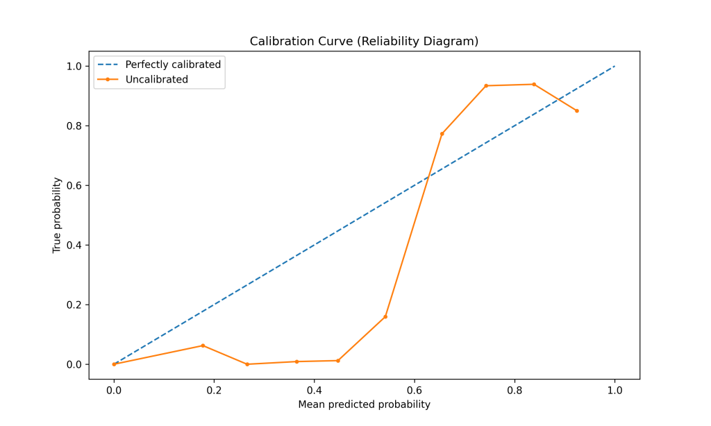
The calibration curve, also known as the reliability diagram, plots the mean predicted probability against the true fraction of positive samples. A perfectly calibrated model would follow the diagonal line, where the x-axis represents the model’s predicted probabilities while the y-axis shows the actual proportion of positive samples for each probability bin.

Did you know that over- or undersampling the training set might distort the calibration of a classifier beyond repair? We discuss a recent article that covers this topic in our free booklet “7 Takes on Working with Imbalanced Data“. Check it out.

Implementing Probability Calibration in Python

Let’s dive into a practical example using Python and scikit-learn to demonstrate probability calibration.

We’ll start by loading the required libraries and creating a function to compute Brier, log loss, and ROC-AUC scores:

import pandas as pd
import matplotlib.pyplot as plt

from sklearn.datasets import make_classification
from sklearn.model_selection import train_test_split
from sklearn.svm import SVC
from sklearn.metrics import roc_auc_score, brier_score_loss, log_loss
from sklearn.calibration import CalibratedClassifierCV, calibration_curve

def compute_scores(y_true, y_pred_proba, name=None):
    """Compute a specific set of classification scores."""
    scores = {
        'brier_score': brier_score_loss(y_true, y_pred_proba),
        'log_loss_score': log_loss(y_true, y_pred_proba),
        'roc_auc': roc_auc_score(y_true, y_pred_proba)
    }
    return pd.Series(scores).rename(name)

Now, let’s create a sample dataset for our binary classification task:

# Generate a binary classification dataset
X, y = make_classification(
    n_samples=10_000, n_classes=2, weights=[0.7, 0.3], random_state=42
)

# Split the data into training and testing sets
X_train, X_test, y_train, y_test = train_test_split(X, y, test_size=0.2, random_state=42)

This code produces a slightly imbalanced dataset (proportions 70:30) and splits it into train and test sets.

As the next step, let’s train an SVM classifier on our toy dataset and get the probability estimates:

# Train an SVM binary classifier (known to produce uncalibrated probabilities)
clf = SVC(kernel='rbf', random_state=42)
clf.fit(X_train, y_train)

# Get probability predictions (uncalibrated)
y_pred_proba = clf.decision_function(X_test)
y_pred_proba = (y_pred_proba - y_pred_proba.min()) / (y_pred_proba.max() - y_pred_proba.min())

Note that I’ve used clf.decision_function , which gives us the raw decision scores from the SVM classifier, followed by a min-max normalization to simulate probability estimates. I’ve decided to use an SVM classifier with an RBF kernel (known to produce uncalibrated probabilities) for didactic purposes. However, many classifiers support the method .predict_proba so we should use it instead whenever available.

Now, let’s compute and plot the calibration curve:

# Calculate calibration curve
prob_true, prob_pred = calibration_curve(y_test, y_pred_proba, n_bins=10)

# Calibration plot
plt.figure(figsize=(10, 6))
plt.plot([0, 1], [0, 1], linestyle='--', label='Perfectly calibrated')
plt.plot(prob_pred, prob_true, marker='.', label='Uncalibrated')
plt.xlabel('Mean predicted probability')
plt.ylabel('True probability')
plt.title('Calibration Curve (Reliability Diagram)')
plt.legend()
plt.show()

In this code, we use calibration_curve to compute the calibration curve. Let’s break down its key parameters:

• n_bins: This parameter determines the number of bins used to calculate the calibration curve. More bins provide a more detailed curve but may be noisier, especially with limited data.
• strategy: This parameter determines how the bins are created. ‘quantile’ ensures that each bin has the same number of samples, which is particularly useful for imbalanced datasets.

In a probability calibration plot, we plot the probability against the actual occurrence of the event. If the probabilities are calibrated, we should expect a straight line. In the following output we see that the probability score is not calibrated, as the yellow line deviates from the dotted blue line, which represents the perfect calibration.

Let’s also compute the target scores using the function we’ve created earlier:

# Compute metrics for predictor
print(compute_scores(y_test, y_pred_proba, name='Uncalibrated'))

We find the values for the different metrics in the following output:

brier_score       0.177542
log_loss_score    0.539588
roc_auc           0.968339

In the following code, we’ll use CalibratedClassifierCV to calibrate the probabilities of our SVM using the methods “sigmoid” and “isotonic” discussed in the section “Understanding Calibration Methods“:

# Calibrate using Platt Scaling
clf_platt = CalibratedClassifierCV(clf, cv=5, method='sigmoid')
clf_platt.fit(X_train, y_train)

# Calibrate using Isotonic Regression
clf_isotonic = CalibratedClassifierCV(clf, cv=5, method='isotonic')
clf_isotonic.fit(X_train, y_train)

# Get calibrated probability predictions for both methods
y_pred_proba_platt = clf_platt.predict_proba(X_test)[:, 1]
y_pred_proba_isotonic = clf_isotonic.predict_proba(X_test)[:, 1]

With the calibrated probabilities, we can now plot the calibration curves for both calibrated methods, including the original uncalibrated curve from our previous code:

# Calculate calibration curves
prob_true, prob_pred_uncal = calibration_curve(
    y_test, y_pred_proba, n_bins=10, strategy='quantile'
)
prob_true_platt, prob_pred_platt = calibration_curve(
    y_test, y_pred_proba_platt, n_bins=10, strategy='quantile'
)
prob_true_isotonic, prob_pred_isotonic = calibration_curve(
    y_test, y_pred_proba_isotonic, n_bins=10, strategy='quantile'
)

# Calibration plot
plt.figure(figsize=(10, 6))
plt.plot([0, 1], [0, 1], linestyle='--', label='Perfectly calibrated')
plt.plot(prob_pred_uncal, prob_true, marker='.', label='Uncalibrated')
plt.plot(prob_pred_platt, prob_true_platt, marker='.', label='Platt Scaling')
plt.plot(prob_pred_isotonic, prob_true_isotonic, marker='.', label='Isotonic Regression')
plt.xlabel('Mean predicted probability')
plt.ylabel('True probability')
plt.title('Calibration Curves Comparison')
plt.legend()
plt.show()

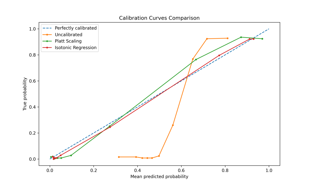
In the following output we see that both Platt scaling and isotonic regression restored the calibration of the probability, as both curves (red and green) now follow more closely the perfectly calibrated blue dotted line:

Let’s compute the target scores to compare them between the uncalibrated and calibrated probability estimates:

# Compute metrics for predictor
df_scores = pd.DataFrame([
    compute_scores(y_test, y_pred_proba, name='Uncalibrated'),
    compute_scores(y_test, y_pred_proba_platt, name='Platt Scaling'),
    compute_scores(y_test, y_pred_proba_isotonic, name='Isotonic Regression')
])
print(df_scores)

The following output shows that, as expected, the model performance (assessed by the ROC-AUC) is similar regardless of probability calibration. However, the Brier score and log loss are noticeably smaller than those returned by the uncalibrated approach:

                     brier_score  log_loss_score   roc_auc
Uncalibrated            0.177542        0.539588  0.968339
Platt Scaling           0.053869        0.202653  0.968106
Isotonic Regression     0.051877        0.188629  0.967950

Note: Note that we have applied CalibratedClassifierCV on the training set. Nonetheless, it’s worth noticing that the calibrator should fit on a dataset independent of the training data used to fit the classifier. A recommendable approach is calibrating the probabilities on a separate validation set (not seen in training) with the fitted model and then evaluating it using the test set.

Calibration for Multi-class Problems

While we’ve focused on binary classification, probability calibration is also applicable to multi-class problems. Scikit-learn’s CalibratedClassifierCV automatically handles multi-class scenarios using a one-vs-rest approach.

Best Practices and Considerations

• Cross-validation: Always use cross-validation when calibrating to prevent overfitting.
• Separate calibration set: If possible, use a separate calibration dataset distinct from your training and testing sets. This approach, known as the “three-way split,” helps prevent overfitting and provides a more reliable estimate of the model’s performance on unseen data.
• Model selection: Remember that calibration doesn’t improve a model’s discriminating power. Select your best model first, then calibrate.
• Recalibration: Periodically recalibrate your model, especially if the data distribution changes over time.
• Visualization: Always visualize your calibration curves to understand how your model’s probabilities are being adjusted.

When Calibration Might Not Help

It’s important to note that probability calibration isn’t always beneficial. There are cases where calibrating probabilities might not improve or even slightly worsen the model’s performance:

1. Already well-calibrated models: If a model is already well-calibrated (e.g., logistic regression in many cases), additional calibration might introduce unnecessary complexity without significant benefits.
2. Small datasets: Calibration might lead to overfitting on small datasets.
3. Extreme class imbalance: In cases of severe class imbalance, calibration methods might struggle to provide reliable probability estimates for the minority class.
4. Non-monotonic relationship: If the relationship between the model’s scores and true probabilities is non-monotonic, methods like Platt Scaling and Isotonic Regression might not capture this complexity accurately.
5. When discriminating power is more important: In some applications, the ranking of predictions might be more important than their absolute probability values. In such cases, focusing on calibration might not be the best use of resources.

Conclusion

Probability calibration is crucial in developing machine learning models with reliable and trustworthy probability estimates. By ensuring that our classifiers’ probability estimates accurately reflect true class probabilities, we enhance their utility in real-world decision-making scenarios.

In this article, we’ve explored the concept of probability calibration, its importance, and how to implement it using Python and scikit-learn. We’ve seen how techniques like Platt Scaling and Isotonic Regression can significantly improve the calibration of our models’ probability estimates.

The next time you work on a classification problem, consider including probability calibration as part of your workflow to create models that not only predict class labels accurately but also provide well-calibrated probabilities that are essential for confident decision-making.

Additional resources

Master probability calibration with out our book Machine Learning with Imbalanced Data: