Class Imbalance in Machine Learning: Definition, Imbalance Ratio and Why It's Rarely the Problem

Class imbalance occurs when the classes of a classification dataset are not equally represented, with one class, the majority class, far outnumbering the other, the minority class. In a credit card fraud dataset, for example, fewer than 2 in every 1,000 transactions are fraudulent.

You’ll often read that class imbalance makes machine learning models perform poorly, and that we need to fix it with class balancing techniques like oversampling, undersampling, SMOTE (Synthetic Minority Oversampling Technique) or class weights. In practice, the real problems usually lie in how we evaluate and configure the models.

In this article, we will cover:

• What class imbalance is, and how to measure it with the imbalance ratio
• Why class imbalance seems to be a problem, and the four issues that actually make imbalanced classification hard
• A Python example with a credit card fraud dataset, where we compare resampling, class weights and threshold tuning, with standard deviations
• A summary of how to handle class imbalance

This article summarizes the first chapter of my book Imbalanced Data: Myths, Mistakes and Modern Solutions, where I test these ideas on dozens of imbalanced datasets and discuss the evidence behind each recommendation.

What Is Class Imbalance?

A dataset has class imbalance when its class distribution is uneven, with some classes appearing far more often than others. The most frequent class is called the majority class, and the rare one, which is usually the one we care about, the minority class.

Datasets with class imbalance are called imbalanced datasets, or class-imbalanced datasets, and you’ll also find the term unbalanced classes. They are common whenever we try to predict rare events.

Class imbalance can happen in binary classification, where the minority class is usually labeled as the positive class, and in multiclass classification. In multiclass problems, we can have one or several majority classes, and one or several minority classes.

Class Imbalance in the Real World

Class imbalance is the norm in many real-world applications:

• Fraud detection: fraudulent transactions are a tiny fraction of all payments.
• Medical diagnosis: most patients don’t have the rare disease we want to detect.
• Customer churn: in a given month, most customers stay.
• Spam detection and defect detection: spam emails and faulty products are a minority.

In all these examples, the minority class is the one we want to find, and missing it is usually costly.

Measuring Class Imbalance: The Imbalance Ratio

The most common way to measure class imbalance is the imbalance ratio, the number of majority class observations divided by the number of minority class observations:

\[\text{IR} = \frac{N_{majority}}{N_{minority}}\]

A dataset with 990 legitimate and 10 fraudulent transactions has an imbalance ratio of 99, that is, 99 majority observations per minority observation. Equivalently, the minority class represents 1% of the data.

When Is a Dataset Imbalanced?

Strictly speaking, any dataset with unequal class proportions is imbalanced, so there is no magic imbalance ratio beyond which models stop working. As we’ll see, model performance depends much more on other factors.

Class Imbalance and Fairness

You may also find the term class imbalance in the context of fairness and bias auditing. There, it refers to the imbalance between groups of people in the training data, for example between age groups, and it is measured to check whether a model may treat some groups unfairly.

That is a different concept from the imbalance between the target classes that we discuss in this article.

The Class Imbalance Problem: What Really Makes Imbalanced Data Hard

The belief in a class imbalance problem comes mostly from two observations. Models trained on imbalanced data seem to have a majority class bias, ignoring the minority class, and their accuracy looks great while they miss most of the cases we care about.

Both observations are real, but their causes are elsewhere. The challenges attributed to class imbalance almost always stem from four more fundamental issues:

1. Using misleading evaluation metrics
2. Having too few minority class examples
3. Poor class separability
4. Choosing the wrong machine learning model

Let’s go through each one.

Problem 1: Misleading Evaluation Metrics

Accuracy, the fraction of correct predictions, is misleading on imbalanced data. On a dataset with 99 majority observations per minority observation, a useless model that always predicts the majority class reaches 99% accuracy, while missing every single minority case. This is known as the accuracy paradox.

Other metrics, like precision, recall and the F1 score, depend on the decision threshold, the probability above which we assign an observation to the minority class. Most libraries use 0.5 by default, which is usually too high for imbalanced data, and makes the model look like it ignores the minority class.

Many studies that promote resampling methods evaluate their models with these metrics at the default threshold of 0.5. In many cases, simply lowering the threshold on a model trained on the original data gives the same improvement, as shown, for example, by Elor and Averbuch-Elor (2022).

To learn more about metrics for imbalanced data, check out our articles on the confusion matrix, precision and recall, precision-recall curves and balanced accuracy.

Problem 2: Too Few Minority Class Examples

What matters for learning is the absolute number of minority class examples, more than their proportion. A model can learn from 5,000 frauds among 5 million transactions, but it will struggle with 20 frauds among 2,000 transactions, even though the second dataset is far less imbalanced.

A practical way to find out whether we have enough data is to plot learning curves, which show how the performance on a validation set changes as we add more training data. If the performance is still rising when we use all the data, it’s worth trying to collect more data, especially minority examples. In computer vision, data augmentation, like rotating or cropping images, can also add useful new examples.

Problem 3: Poor Class Separability

Class separability describes how distinct the observations of each class are, given the available features. If the features separate the classes well, most models will classify them correctly, even with a thousand majority observations per minority observation.

If the classes overlap, no model will separate them well, whether the data is balanced or not. In that case, the way forward is to engineer better features.

Problem 4: The Wrong Machine Learning Model

Simple models, like logistic regression or decision trees, can’t capture complex patterns, while ensemble methods, like random forests and gradient boosting machines, can. If the minority class lives in a small, irregular region of the feature space, they will miss it, which is a problem of model capacity.

With modern gradient boosting machines like XGBoost or CatBoost, the benefits of resampling largely disappear: Elor and Averbuch-Elor (2022) found that SMOTE improved weak classifiers, but offered no benefit to strong ones. We discuss where the advice to rebalance the data came from in our article on machine learning with imbalanced data.

In chapter 1 of my book, I compare nine models on 35 imbalanced datasets, show how to plot learning curves to check whether you have enough data, and explain why resampling methods became so popular.

Class Imbalance in Python: A Fraud Detection Example

Let’s put this to the test with the credit card fraud dataset, which contains 284,807 transactions made by European cardholders, of which only 492 are fraudulent.

We will compare models trained on the original data, with class weights and with SMOTE, and evaluate them with cross-validation, reporting the mean and standard deviation of each metric. A difference between two models only means something if it is larger than the variability of the estimate.

Loading the Imbalanced Dataset

Let’s import the libraries:

import numpy as np
import pandas as pd
import matplotlib.pyplot as plt
from imblearn.over_sampling import SMOTE
from imblearn.pipeline import make_pipeline
from sklearn.datasets import fetch_openml
from sklearn.dummy import DummyClassifier
from sklearn.ensemble import HistGradientBoostingClassifier
from sklearn.metrics import accuracy_score, precision_score, recall_score
from sklearn.model_selection import (
    StratifiedKFold, cross_validate, train_test_split,
)

Now, we load the dataset from OpenML and count the observations in each class:

data = fetch_openml(name="creditcard", version=1, as_frame=True, parser="auto")
X = data.data
y = data.target.astype(int)

print(y.value_counts())

In the following output, we see the number of legitimate transactions, class 0, and fraudulent ones, class 1:

Class
0    284315
1       492
Name: count, dtype: int64

Let’s calculate the fraction of fraud and the imbalance ratio:

n_majority, n_minority = np.bincount(y)

print(f"Fraction of fraud: {n_minority / len(y):.4f}")
print(f"Imbalance ratio: {n_majority / n_minority:.0f}")

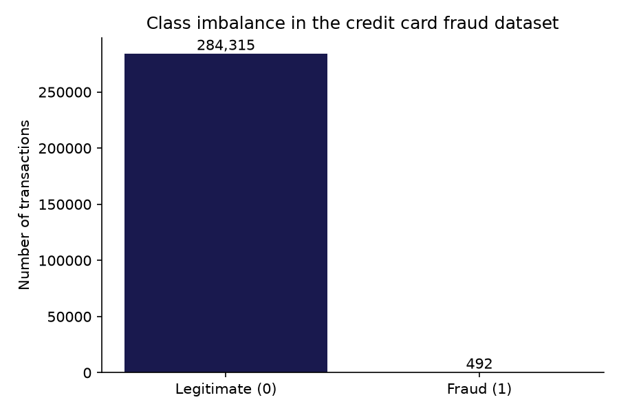
The output shows that only 0.17% of the transactions are fraudulent, which gives an imbalance ratio of 578:

Fraction of fraud: 0.0017
Imbalance ratio: 578

Let’s plot the class distribution:

counts = y.value_counts().sort_index()

fig, ax = plt.subplots(figsize=(6, 4))
bars = ax.bar(["Legitimate (0)", "Fraud (1)"], counts.values)
ax.bar_label(bars, labels=[f"{v:,}" for v in counts.values])
ax.set_ylabel("Number of transactions")
ax.set_title("Class imbalance in the credit card fraud dataset")
plt.show()

In the following bar plot, the fraudulent transactions are barely visible next to the legitimate ones:

The Accuracy Paradox in Practice

Next, we split the data into a training and a test set. With stratify=y, both sets keep the same fraction of fraud, which is essential with imbalanced data, because a random split could leave very few frauds in the test set:

X_train, X_test, y_train, y_test = train_test_split(
    X, y, test_size=0.3, random_state=0, stratify=y,
)

Let’s evaluate a dummy model that always predicts the majority class:

dummy = DummyClassifier(strategy="most_frequent").fit(X_train, y_train)
y_pred = dummy.predict(X_test)

print(f"Accuracy: {accuracy_score(y_test, y_pred):.4f}")
print(f"Recall:   {recall_score(y_test, y_pred):.4f}")

The output shows the accuracy paradox:

Accuracy: 0.9983
Recall:   0.0000

The dummy model is 99.83% accurate, and it doesn’t catch a single fraud. That’s why, for the rest of this demo, we will use metrics that focus on how well the models find the minority class.

Comparing Class Weights and SMOTE With Cross-Validation

We will evaluate the models with three metrics:

• ROC-AUC: how well the model ranks frauds above legitimate transactions, across all thresholds.
• Average precision: the area under the precision-recall curve, which focuses on the minority class.
• Brier score: the mean squared difference between the predicted probabilities and the real outcomes, which tells us whether the probabilities can be trusted. Lower is better.

None of them depends on the decision threshold, so they measure the models themselves. We compare five gradient boosting machines, with and without regularization, class weights and SMOTE:

cv = StratifiedKFold(n_splits=5, shuffle=True, random_state=0)

models = {
    "Default": HistGradientBoostingClassifier(random_state=0),
    "Default + class weights": HistGradientBoostingClassifier(
        class_weight="balanced", random_state=0),
    "Regularized": HistGradientBoostingClassifier(
        l2_regularization=1.0, random_state=0),
    "Regularized + class weights": HistGradientBoostingClassifier(
        l2_regularization=1.0, class_weight="balanced", random_state=0),
    "Regularized + SMOTE": make_pipeline(
        SMOTE(random_state=0),
        HistGradientBoostingClassifier(l2_regularization=1.0, random_state=0)),
}

results = {}
for name, model in models.items():
    cv_res = cross_validate(
        model, X, y, cv=cv,
        scoring=["roc_auc", "average_precision", "neg_brier_score"],
    )
    roc = cv_res["test_roc_auc"]
    ap = cv_res["test_average_precision"]
    brier = -cv_res["test_neg_brier_score"]
    results[name] = {
        "ROC-AUC": f"{roc.mean():.3f} ± {roc.std():.3f}",
        "Average precision": f"{ap.mean():.3f} ± {ap.std():.3f}",
        "Brier score": f"{brier.mean():.5f} ± {brier.std():.5f}",
    }

print(pd.DataFrame(results).T.to_string())

Note that we use imbalanced-learn’s make_pipeline for SMOTE, so that the synthetic data is created only from the training folds, and never from the data we evaluate on.

In the following output, we see the mean and standard deviation of each metric across the 5 folds:

                                   ROC-AUC Average precision        Brier score
Default                      0.788 ± 0.048     0.620 ± 0.034  0.00147 ± 0.00017
Default + class weights      0.966 ± 0.014     0.756 ± 0.031  0.00255 ± 0.00043
Regularized                  0.978 ± 0.011     0.842 ± 0.012  0.00043 ± 0.00002
Regularized + class weights  0.969 ± 0.015     0.756 ± 0.031  0.00279 ± 0.00080
Regularized + SMOTE          0.981 ± 0.008     0.853 ± 0.015  0.00104 ± 0.00008

Class Weights Hid a Model Configuration Problem

Look at the first two rows. With its default settings, the gradient boosting machine has a poor ROC-AUC of 0.788, and adding class weights raises it to 0.966. It looks like the class imbalance was the problem, and class weights fixed it.

The third row tells a different story. Adding a small amount of L2 regularization to the model, without touching the data, raises the ROC-AUC to 0.978 and the average precision to 0.842, better than any of the default models.

Why does this happen? Gradient boosting sets the value of each leaf by dividing the sum of the gradients by the sum of the second derivatives of the loss, and with probabilities close to zero, as they are for the rare class, those second derivatives become tiny. Leaves with a handful of frauds then get extreme values, and the model becomes unstable.

L2 regularization adds a constant to that denominator, while class weights inflate the second derivatives of the frauds, which is why both appear to fix the problem.

In my tests, XGBoost and LightGBM with their default settings were also unstable on this dataset. So, the problem was the configuration of the model, which brings us back to Problem 4.

Class Weights and SMOTE Don’t Improve a Well-Configured Model

Now compare the regularized model with its versions trained with class weights and with SMOTE. The ROC-AUC of the three is the same within one standard deviation, so neither class weights nor SMOTE made the model better at separating frauds from legitimate transactions.

The average precision tells the same story for SMOTE, while class weights made it worse. And both made the probabilities less reliable: the Brier score is about 2.4 times higher with SMOTE, and more than 6 times higher with class weights.

That’s because resampling and class weights make the model believe that frauds are much more frequent than they really are, so it overestimates their probability. We discuss this in our article on probability calibration.

Studies on clinical risk prediction reached the same conclusion: van den Goorbergh and colleagues (2022) found that correcting for class imbalance made the models’ probabilities worse without improving their discrimination.

Adjusting the Decision Threshold Instead of Resampling

If SMOTE doesn’t make the model better, why do so many tutorials show it improving the recall? Let’s check by training the regularized model on the original training set, and calculating precision and recall at different thresholds on the test set:

model = HistGradientBoostingClassifier(l2_regularization=1.0, random_state=0)
model.fit(X_train, y_train)
probs = model.predict_proba(X_test)[:, 1]

rows = []
for t in [0.5, 0.2, 0.05, 0.02, 0.01, 0.005]:
    pred = (probs >= t).astype(int)
    rows.append({
        "threshold": t,
        "precision": precision_score(y_test, pred),
        "recall": recall_score(y_test, pred),
    })

print(pd.DataFrame(rows).round(3).to_string(index=False))

In the following output, we see that lowering the threshold catches more frauds, at the price of more false alarms:

 threshold  precision  recall
     0.500      0.926   0.757
     0.200      0.890   0.764
     0.050      0.812   0.791
     0.020      0.709   0.824
     0.010      0.644   0.831
     0.005      0.544   0.838

Now, let’s train the same model on data rebalanced with SMOTE, and evaluate it at the default threshold of 0.5:

smote_model = make_pipeline(
    SMOTE(random_state=0),
    HistGradientBoostingClassifier(l2_regularization=1.0, random_state=0),
)
smote_model.fit(X_train, y_train)
y_pred_smote = smote_model.predict(X_test)

print(f"SMOTE at 0.5  precision: {precision_score(y_test, y_pred_smote):.3f}  "
      f"recall: {recall_score(y_test, y_pred_smote):.3f}")

The output shows the precision and recall of the SMOTE model:

SMOTE at 0.5  precision: 0.649  recall: 0.851

The model trained on the original data reaches the same precision, 0.644, at a threshold of 0.01, with a recall of 0.831. That’s a difference of only 3 out of 148 frauds in the test set.

In other words, SMOTE moved the decision boundary, so that the default threshold of 0.5 behaves like a much lower threshold on the original model. We can get the same effect by choosing the threshold directly, which is simpler and keeps the probabilities intact.

The following plot shows the full trade-off between precision and recall for the model trained on the original data:

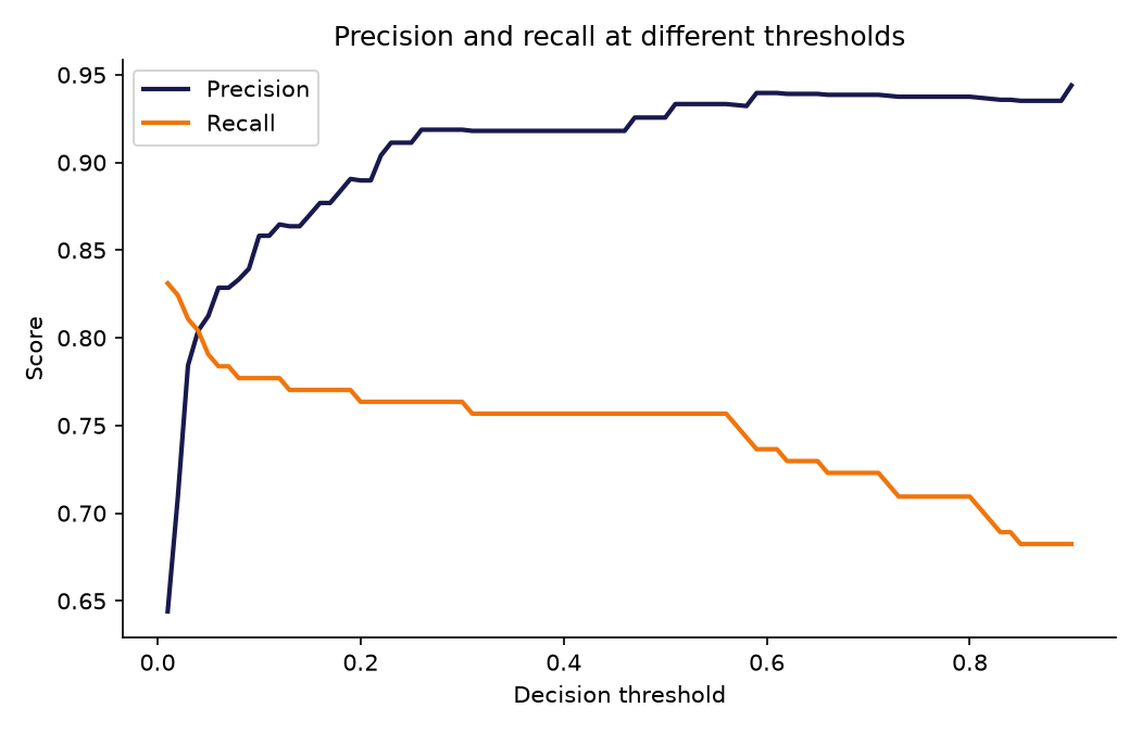
This is often called threshold moving. By moving the threshold, we can pick any point on this trade-off according to the misclassification cost of missing a fraud versus investigating a legitimate transaction. We show how to tune the threshold with scikit-learn’s TunedThresholdClassifierCV in our article on cost-sensitive learning.

How to Handle Class Imbalance: A Summary

The demo points to a simple approach when the classes are imbalanced:

• Train a strong, well-configured model on the original data, tuning its hyperparameters, including regularization, as you would for any other dataset.
• Evaluate it with the right metrics: threshold-independent metrics like the ROC-AUC or the average precision, and proper scoring rules like the Brier score, with their standard deviation across stratified cross-validation folds.
• Think in probabilities: decisions are often left to domain experts, who need calibrated probabilities, as Frank Harrell explains in his post on classification vs prediction.
• Tune the decision threshold to the costs of your problem when you need class labels.
• Check whether you need more data with learning curves, before trying anything else.
• Consider anomaly detection when the minority class is extremely rare and you have very few labeled examples of it.

Resampling and class weights keep a few legitimate uses, like random undersampling to speed up training on very large datasets, or weights to encode real costs. Random oversampling and SMOTE are a last resort for tiny minority classes, keeping in mind that duplicating observations can lead to overfitting and that synthetic data may not be realistic. You can learn more about them in our articles on undersampling, oversampling, SMOTE and ADASYN.

For a step-by-step guide to the techniques and best practices, including evaluation metrics, calibration, cost-sensitive learning, resampling and ensembles, check out our article on machine learning with imbalanced data.

Myths, Mistakes and Modern Solutions

Myth: imbalanced classes are an inherent problem for classification. The challenges usually come from too few minority examples, overlapping classes, or the use of inappropriate models and metrics.

Mistakes: evaluating models with threshold-dependent metrics at the default threshold of 0.5, comparing models with single numbers without their variability, and assuming that results obtained with simple models hold for modern gradient boosting machines.

Modern solution: use strong, well-tuned classifiers trained on the original data, evaluate them with threshold-independent metrics and proper scoring rules, and tune the decision threshold to the costs of your problem.

Frequently Asked Questions About Class Imbalance

What is class imbalance in machine learning?

Class imbalance occurs when the classes of a classification dataset are not equally represented, so one class, the minority class, has far fewer observations than the others. It is common in fraud detection, medical diagnosis and churn prediction.

How do you measure class imbalance?

The most common measure is the imbalance ratio, the number of majority class observations divided by the number of minority class observations. You can also report the fraction of observations in the minority class.

Does class imbalance always hurt model performance?

No. Strong models can separate imbalanced classes well when the features are informative and there are enough minority examples. What usually hurts is evaluating the models with accuracy, or with precision and recall at the default threshold of 0.5.

Does class imbalance affect deep learning?

The same principles apply. Deep learning models also need enough minority examples and the right metrics, and research on convolutional neural networks has found them more sensitive to small datasets than to the imbalance ratio itself.

Should I use SMOTE to handle class imbalance?

Try adjusting the decision threshold first. SMOTE and other resampling methods shift the decision boundary, which is equivalent to lowering the threshold, and they distort the predicted probabilities.

Conclusion

Class imbalance describes datasets where one class far outnumbers the other, and we can measure it with the imbalance ratio. It is everywhere in real applications, but it is rarely what makes a classification problem hard.

Misleading metrics, too few minority examples, overlapping classes and poorly chosen or poorly configured models are the real culprits. Train a strong model on the original data, evaluate it with the right metrics and their variability, and tune the decision threshold to your costs.

If you want to see the evidence behind these recommendations, with experiments on dozens of datasets and chapters on metrics, calibration, cost-sensitive learning, undersampling and oversampling, check out my book Imbalanced Data: Myths, Mistakes and Modern Solutions.

References

• Elor and Averbuch-Elor. 2022. To SMOTE, or Not to SMOTE? arXiv.
• van den Goorbergh, van Smeden, Timmerman and Van Calster. 2022. The Harm of Class Imbalance Corrections for Risk Prediction Models. Journal of the American Medical Informatics Association.
• Provost. 2000. Machine Learning From Imbalanced Data Sets 101. Proceedings of the AAAI Workshop on Imbalanced Data Sets.
• Scikit-learn documentation: HistGradientBoostingClassifier.