
Multiple Imputation with Chained Equations (MICE) – what is it?
In many real-world data science projects, data scientists, spend up to 80% of their time on data preparation involving data processing, cleaning, and organizing data into structures that can be further analyzed. This includes preparing a complete dataset, which consists of filling in missing values with estimates – a difficult challenge to address.
Choosing appropriate imputation methods is crucial to maintaining consistent data distributions. Missing data often occurs in independent variables for various reasons, such as, human error, data entry problems, or equipment malfunctions during data collection.
Most of machine learning models expect the data to be complete without any trace of null values. Rows with missing data points can detrimentally affect the models’ predictive power, introducing bias, reducing the model’s accuracy and making some statistical analyses inapplicable. This is why it is essential to tackle missing data effectively.
The act of replacing missing values by estimates, is called missing data imputation. Imputation methods are divided in 2 categories: univariate imputation and multivariate imputation. Let’s begin by reviewing univariate imputation.
Univariate Imputation
Univariate imputation methods consist of replacing missing values with statistical estimates obtained from the observed data on a single variable. For example, we can replace missing values in numerical variables with the mean or the median of the observed values, or replace missing data in categorical variables with the most frequent category or an arbitrary (constant) value.
Many data scientists use univariate imputation techniques due to its simplicity when they want to obtain complete datasets fast. These methods, however, do not always translate well into inference predictions made from regression models, in particularly when the proportion of missing data is large or the data is not MCAR (missing completely at random).

Multivariate imputation of chained equations (MICE)
Stef van Buuren introduced Multiple Imputation by Chained Equations (MICE) to overcome the limitation of missing data in univariate perspectives.
The MICE algorithm offers a robust method of imputing values through iterative estimations based on conditional distributions. It accounts for dependencies between variables, by using the values of other variables to estimate the missing data.
How MICE operates step-by-step:
- Initial Imputation: Fill in all the missing values in the dataset with simple placeholders, for example the mean or median of each variable (for categorical type, the most frequent will do).
- Reset Missing Values: Next, choose one variable at a time for imputation, and change those placeholder values back to missing.
- Build Regression Model: Build a regression model to predict the variable from step 2, by using the other independent variables in the dataset. This model uses all (or some) of the other variables in the dataset as predictors to estimate the values of the missing data points.
- Replace Missing Values: Use the regression model to predict and fill in the missing values for this variable. At this point, this variable has now both observed and newly imputed values.
- Repeat for Each Variable: Repeat steps 2-4 for every variable in the dataset that has missing values.
Going through all the variables will complete one iteration or “cycle.”
Repeat steps 2-4 for several cycles. For each cycle, the model updates imputation values, making the predictions more accurate. In general, after 10 cycles, the model is said to have reached convergence and the estimates don’t improve any further.
To learn more about MICE and other imputation methods, check out our course Feature Engineering for Machine Learning.

MICE imputation: advantages and limitations
The methodology of MICE comes with benefits:
- Effectively handle missing data multivariate: MICE can handle datasets with a high proportion of missing values by creating multiple imputations, which makes it a robust method for dealing with incomplete data.
- Maintains Data Variability: MICE preserves the natural variability and relationships within the data, leading to more accurate and reliable results.
- Versatile: It can be applied to various types of data, including continuous, categorical, and mixed data types, making it widely applicable in different fields. At least in theory.
- Reduces Bias: MICE reduces bias that can occur with single imputation methods by examining the uncertainty associated with the missing data.
- Improves Predictive Power: By properly addressing missing data, MICE can improve the performance and predictive power of machine learning models.
On the other side, there are also limitations that we have to address:
- Computationally Intensive: MICE requires significant computational resources and time, especially for large datasets with many variables and missing values.
- Complexity: Implementing and tuning MICE can be complex and requires a good understanding of the method, which can be a barrier for practitioners with less experience.
- Assumptions: MICE relies on the assumption that the data is missing at random (MAR), which may not always hold true. If data is missing not at random (MNAR), the imputation results may be biased.
- Model Dependency: The quality of imputations depends on the chosen imputation models for each variable. Poorly chosen models can lead to inaccurate imputations.
- Software Limitations: Not all statistical software packages fully support MICE, which can limit its accessibility and usability for some users.
If you want to apply MICE with R, you can use the mice package. In Python, we have Scikit-learn’s IterativeImputer, which comes with some limitations.
To learn more about MICE and other imputation methods, check out our Python Feature Engineering Cookbook (also available on Amazon).

MICE imputation in Python
In Python, MICE is available through the IterativeImputer from scikit-learn. Let’s demonstrate how it works in code. First, we import libraries needed to do the task:
import numpy as np
import pandas as pd
import matplotlib.pyplot as plt

from sklearn.experimental import enable_iterative_imputer
from sklearn.impute import IterativeImputer, SimpleImputer
from sklearn.linear_model import PoissonRegressor
We load the horse colic dataset from the UCI machine learning repository. Fortunately, we can directly import datasets from the repository to our notebooks. You just need to install the ucimlrepo package by executing !pip install ucimlrepo from the notebook before running the following commands.
from ucimlrepo import fetch_ucirepo
horse_colic = fetch_ucirepo(id=47)
X = horse_colic.data.features
As there are many features with missing data, we select some columns in integer format:
vars = [
    'surgery',
    'temperature_of_extremities',
    'peripheral_pulse',
    'mucous_membranes',
    'capillary_refill_time',
    'pain',
    'peristalsis',
    'abdominal_distension',
    'nasogastric_reflux',
    'rectal_examination_feces',
    'abdomen',
    'abdominocentesis_appearance',
    'outcome'
]

X = X[vars]
print(X.head())
In the following output we see the resulting dataset:
   surgery  temperature_of_extremities  peripheral_pulse  mucous_membranes  \
0      2.0                         3.0               3.0               NaN
1      1.0                         NaN               NaN               4.0
2      2.0                         1.0               1.0               3.0
3      1.0                         4.0               1.0               6.0
4      2.0                         NaN               NaN               6.0

   capillary_refill_time  pain  peristalsis  abdominal_distension  \
0                    2.0   5.0          4.0                   4.0
1                    1.0   3.0          4.0                   2.0
2                    1.0   3.0          3.0                   1.0
3                    2.0   2.0          4.0                   4.0
4                    2.0   NaN          NaN                   NaN

   nasogastric_reflux  rectal_examination_feces  abdomen  \
0                 NaN                       3.0      5.0
1                 NaN                       4.0      2.0
2                 NaN                       1.0      1.0
3                 2.0                       3.0      NaN
4                 NaN                       NaN      NaN

   abdominocentesis_appearance  outcome
0                          NaN      2.0
1                          2.0      3.0
2                          NaN      1.0
3                          3.0      2.0
4                          NaN      2.0
We calculate the proportion of missing data on each feature:
X.isnull().mean()
In the following output we see the fraction of missing values per variable:
surgery                        0.005435
temperature_of_extremities     0.176630
peripheral_pulse               0.225543
mucous_membranes               0.130435
capillary_refill_time          0.103261
pain                           0.171196
peristalsis                    0.141304
abdominal_distension           0.176630
nasogastric_reflux             0.361413
rectal_examination_feces       0.347826
abdomen                        0.388587
abdominocentesis_appearance    0.527174
outcome                        0.005435
dtype: float64
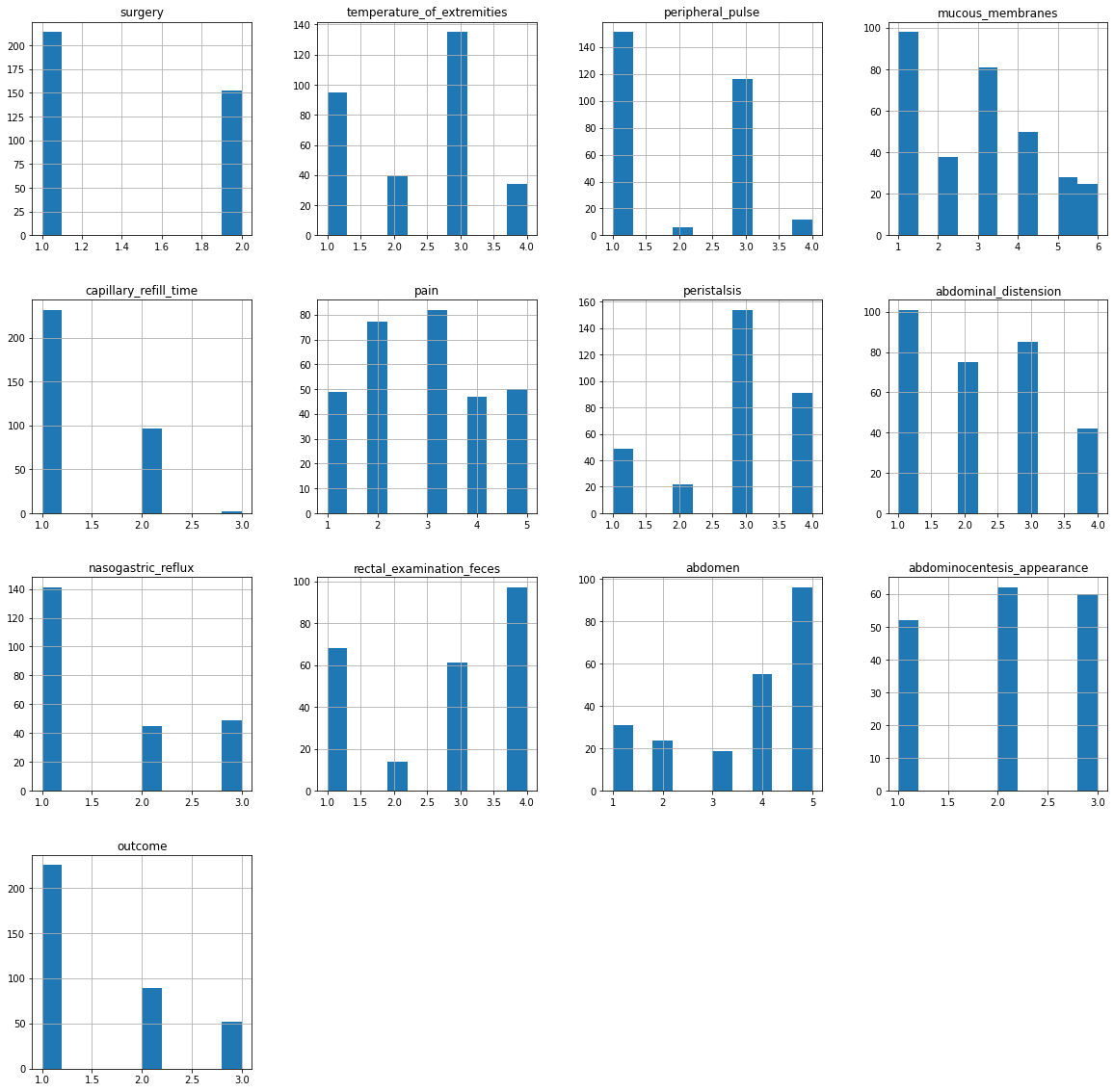
Let’s plot the variables to check out their distribution in the original dataset:
X.hist(figsize=(20,20))
plt.show()
In the following plot we see that the variables are discrete:
We’ll use MICE and together with Poission Regression as an estimator, to obtain values for the imputation. The iterative imputer has several parameters. With initial_strategy, we choose how to set up the missing data to a numeric value in the first round. Here, we replace missing values with the variable mean. With imputation_order, we set up the order in which the variable’s missing data points will be estimated. We start by estimating the values of those variables with less missing data.
To reduce computational cost, by setting skip_complete=True, we’ll only estimate the values of variables with missing data. In our case, it’s all the variables.
imputer = IterativeImputer(
    estimator=PoissonRegressor(solver="newton-cholesky"),
    initial_strategy='mean',
    max_iter=50,
    imputation_order='ascending',
    n_nearest_features=None,
    skip_complete=True,
    random_state=0,
).set_output(transform="pandas")
The parameter max_iter, regulates the number of iterations, that is, how many times the algorithm will execute the steps 2-4 that we described in the previous section. Finally, the set_output method makes the imputer return a dataframe, instead of the default numpy array.
Now, we fit the IterativeImputer paired with PoissonRegressor to the train set to begin the process of parameter building.
imputer.fit(X)
Finally, we use the predicted values to replace missing data by using the transform method.
X_t = imputer.transform(X)
print(X_t.head())
In the following display we see the complete dataset:
   surgery  temperature_of_extremities  peripheral_pulse  mucous_membranes  \
0      2.0                    3.000000          3.000000          4.333889
1      1.0                    2.694633          2.178082          4.000000
2      2.0                    1.000000          1.000000          3.000000
3      1.0                    4.000000          1.000000          6.000000
4      2.0                    2.940653          2.669146          6.000000

   capillary_refill_time      pain  peristalsis  abdominal_distension  \
0                    2.0  5.000000     4.000000               4.00000
1                    1.0  3.000000     4.000000               2.00000
2                    1.0  3.000000     3.000000               1.00000
3                    2.0  2.000000     4.000000               4.00000
4                    2.0  3.395779     3.389313               2.52061

   nasogastric_reflux  rectal_examination_feces   abdomen  \
0            1.802717                  3.000000  5.000000
1            1.993521                  4.000000  2.000000
2            1.479924                  1.000000  1.000000
3            2.000000                  3.000000  4.452293
4            1.888100                  3.084016  3.778047

   abdominocentesis_appearance  outcome
0                     2.425876      2.0
1                     2.000000      3.0
2                     1.509725      1.0
3                     3.000000      2.0
4                     2.478511      2.0
Before moving forward, is worth highlighting that here we fit and transformed the MICE algorithm using the same dataset. For proper data analysis and model evaluation, you want to split the data into a training and testing set, fit the model to the train set, and then evaluate the imputation using the test set.
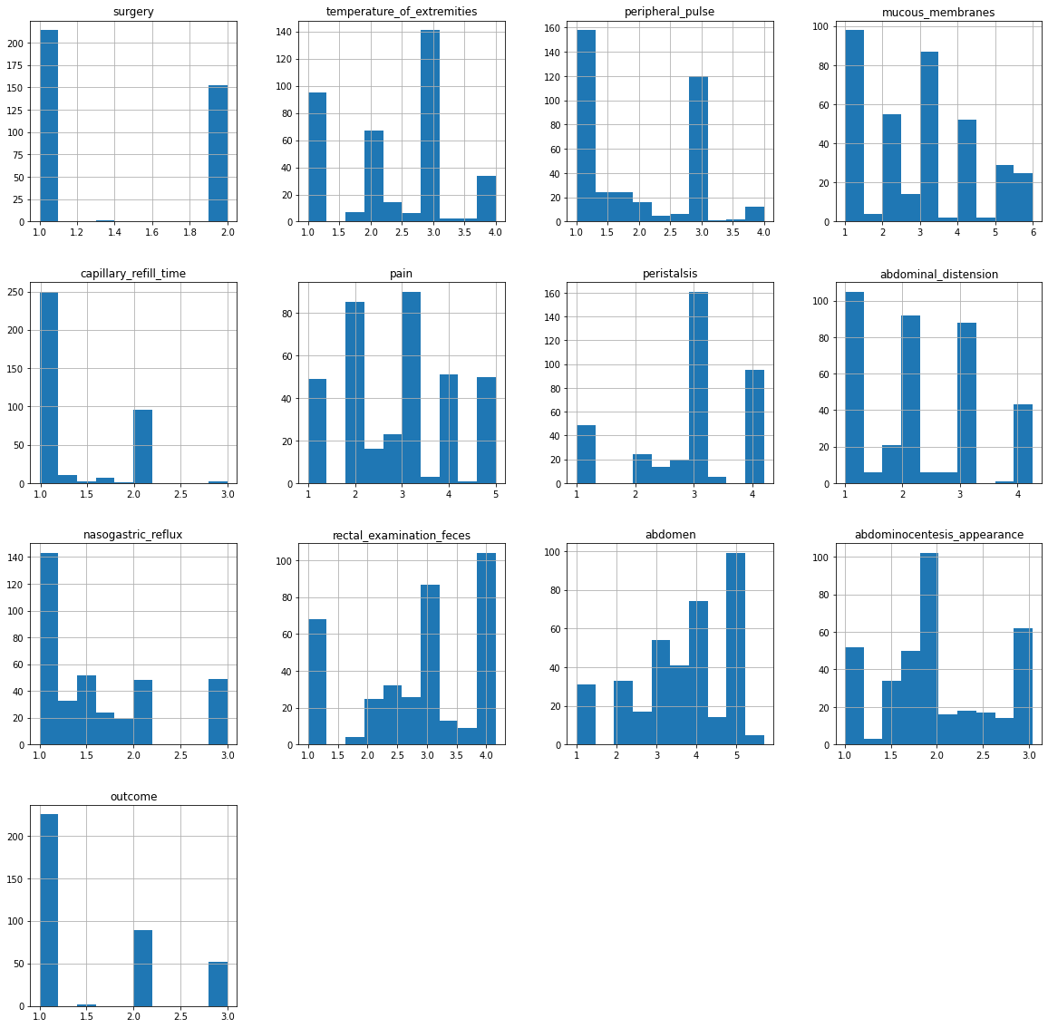
We can go ahead and check the distribution of the variables in the imputed dataset:
X_t.hist(figsize=(20,20))
plt.show()
in the following plot we see the distribution of the variables in the complete dataset:
IterativeImputer accepts any machine learning model for regression, like for example, linear regression, logistic regression (for discrete variables) and random forest, among others.
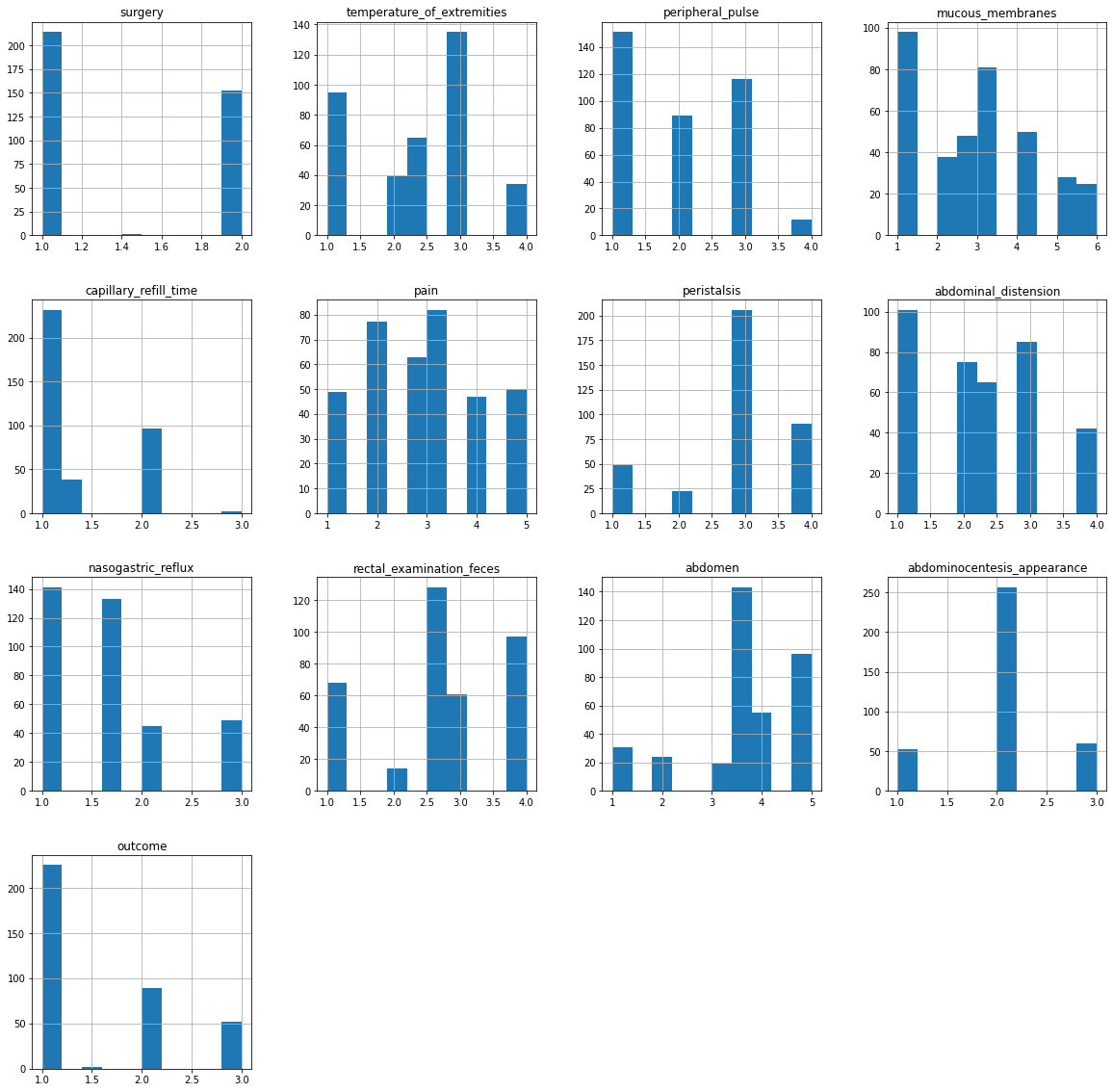
To wrap up our demo of imputation of missing data, we’ll compare the distribution of the variables after replacing null values with an univariate imputation method, for example mean imputation:
imputer = SimpleImputer().set_output(transform="pandas")
X_t = imputer.fit_transform(X)
X_t.hist(figsize=(20,20))
plt.show()
In the following image, we see the variable distrubution after univariate imputation.
MICE, through iterative updates of imputed values using conditional distributions, offers a robust and flexible framework. It outperforms simpler imputation methods in obtaining better estimates of the missing values, making it especially valuable for datasets with complex missing data patterns, leading to more accurate and reliable statistical analyses.
MICE tries to preserve the original variable distribution and the relationship of the variables to its covariates. Simple univariate imputation methods distort the variable distribution and covariance on the other hand.
Resources
If you want to learn more about mice imputation or other missing value imputation methods, check out the following hands-on resources:
