Moving Average Forecasting: What You Need to Know

Moving average forecasting is one of the simplest methods to forecast future values of a time series.

The moving average method works by taking the average of past data points over a chosen number of periods, and then uses that as the forecast value for the next period. By taking the average, moving average smooths short-term fluctuations and highlights long-term trends in time series data.

Because it is easy to apply and understand, the moving average model is often the first forecasting technique used before moving to advanced methods like ARIMA, Holt, or exponential smoothing. Businesses use it for sales forecasting, traders track stock prices, and supply chains rely on it to manage demand.

In this article, we’ll explore moving average forecasting in detail and show you how to apply it in python.

To master more advanced forecasting techniques, check out our course Forecasting with Machine Learning.

Before diving into moving average forecasting, let’s understand what time series data is and why fluctuations make forecasting challenging.

Time Series and Fluctuations

A time series is simply data collected over time—like daily sales, weekly stock prices, or monthly temperatures. Each data point shows the value of something at a given moment.

Time series usually have a few key patterns:

• Trend: the long-term direction, such as a café’s sales steadily growing.
• Seasonality: repeating cycles, like ice cream sales peaking every summer.
• Volatility: sudden changes, such as a spike during a flash sale.
• Noise: small random ups and downs with no real pattern.

These patterns make forecasting challenging. For example, a rainy day might cause one store’s sales to drop sharply, but that doesn’t mean business is declining overall.

These short-term ups and downs in the time series data, which may come from volatility (large irregular changes) or from noise (small random variations) are called Fluctuations.

It turns out, moving average is great at handling these fluctuations. In fact, moving average can smooth out these fluctuations, so we can focus on the real trends. By simplifying the data, moving average make time series analysis and forecasting much clearer.

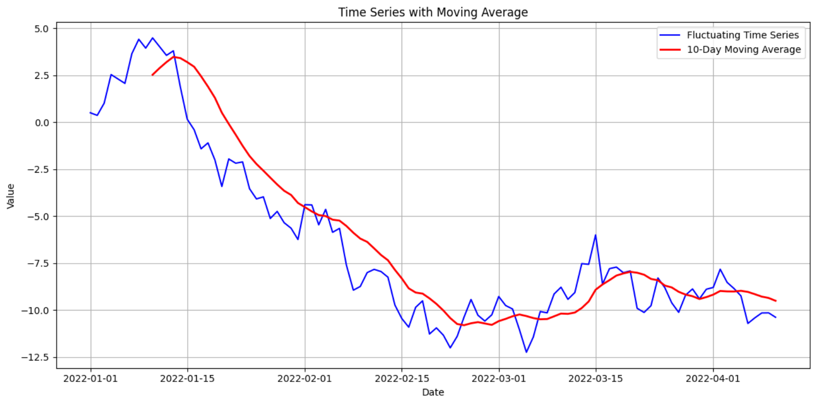
Figure containing a fluctuating time series and a 10-day moving average approximation overlaid.

Now that we understand time series and its fluctuations, let’s discuss moving averages and how they help turn noisy time series data into actionable forecasts.

Moving Average Models

At its simplest, a moving average is just an average of a subset of data points in a time series. Think of it as a sliding window that moves across your dataset, calculating the mean for each time period. By doing this, we smooth out sudden spikes or dips and gain a clearer view of the underlying patterns.

The following image represents how moving average apply to a time series data, the average is taken of the values within the light blue window, and used as the forecast for the period after the window:

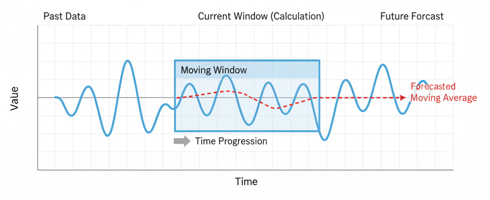
Moving Average Calculation: we take the average of the time series values within a time window, and use that value to predict the next time point.

There are several types of moving averages, each suitable for different forecasting scenarios. Let’s talk about that.

Simple Moving Average (SMA)

The Simple Moving Average, or SMA, is the simplest type of moving average. SMA just takes the mean of a set of continuous data points in the time series and uses that as the forecast value.

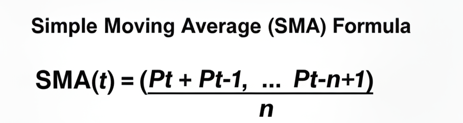
Where:

t = current time period (Eg. 3 days) n = total time period (eg. 5 days) SMA(t) = Simple Moving Average for the current time period Pt = Value at the current time period (eg. $50)

For instance, a retail store tracks its daily sales for one week: 50, 60, 55, 65, 70, 80, and 75 units. If the manager wants to forecast sales for the next day using a 3-day SMA, they would take the last three days of sales—70, 80, and 75—add them up (225), and divide by 3. The SMA forecast for the next day would be 75 units.

SMA works well when the data is relatively stable, without sudden jumps or seasonality.

Now imagine the same store runs a flash discount on the eighth day and sales jump to 150 units, followed by a return to normal levels of 70 and 65 units in the following days. If the manager calculates the SMA with the last three days of sales (150, 70, and 65), the forecast for the next day would be (150 + 70 + 65) ÷ 3 = 285 ÷ 3 = 95 units.

This forecast value of 95 is much higher than the true underlying demand, which was closer to 65–70 units before the promotion. The spike caused the SMA to lag, leading to a significant forecast error.

This example highlights one of SMA’s biggest weaknesses: it cannot easily adapt to sudden, short-term shocks, because it weighs all data points equally, regardless of whether they represent normal demand or an exceptional event.

One solution, would be to use a wider window to calculate the average, the downside being that older data points may not represent well the latest trend. Alternatively, we could use weighted moving average.

We discuss Moving Average, its advantages and shortcomings in detail, and how to leverage it to create features for forecasting wit regression models in our course Feature Engineering for Time Series Forecasting.

Weighted Moving Average (WMA)

The Weighted Moving Average or WMA improves on SMA by giving more importance to recent data points. WMA is simply the weighted average of the data points, as shown in this formula:

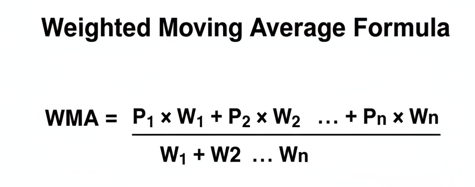
Where:

WMA = Weighed Moving Average P = Value at the current time W = Weight attached to the value at the current time n = total time period

Returning to the earlier retail sales example, if the last three days of sales were 150, 70, and 65 units, and we applied weights of 1, 2, and 3 (where 3 is assigned to the most recent day), the calculation would be: (150×1 + 70×2 + 65×3) ÷ (1+2+3) = (150 + 140 + 195) ÷ 6 = 485 ÷ 6 ≈ 80.8 units.

While this forecast is still somewhat inflated compared to true demand, it is noticeably lower than the SMA forecast of 95 units. This demonstrates how WMA reduces the influence of unusual spikes, by letting more recent, stable values dominate the calculation.

In a Weighted Moving Average, weights are assigned to past observations to reflect their relative importance. Typically, the most recent data gets the highest weight, since it better represents current conditions. The weights can be:

• Linear (e.g., 1, 2, 3, …), where each step closer to the present increases importance.
• Custom (e.g., based on domain knowledge, seasonality, or business rules).
• Normalized (weights add up to 1, e.g., 0.1, 0.3, 0.6) to make interpretation easier.

In the example above, we used a simple linear scheme: 1 for the oldest day, 2 for the middle day, and 3 for the most recent day.

Note however that WMA still risks overreacting when unusual values appear within the most recent time periods. For example, if another flash discount occurs and sales go to 150 instead of 65 on the last day, then the WMA for the same 3 day duration would be (150×1 + 70×2 + 150×3) ÷ (1+2+3) = (150 + 140 + 450) ÷ 6 = 485 ÷ 6 ≈ 123 units. This exaggerates the importance of that spike or fluctuation even more than SMA.

Exponential Moving Average (EMA)

The Exponential Moving Average or EMA, offers a refinement over WMA: Instead of assigning fixed weights, it applies exponentially decreasing weights as observations get older.

EMA does so smoothly with a single parameter, k, rather than explicit weights for each day, like in WMA. This parameter is called the smoothing factor. This way, most recent sales figures dominate, while older data still contributes, but with less influence.

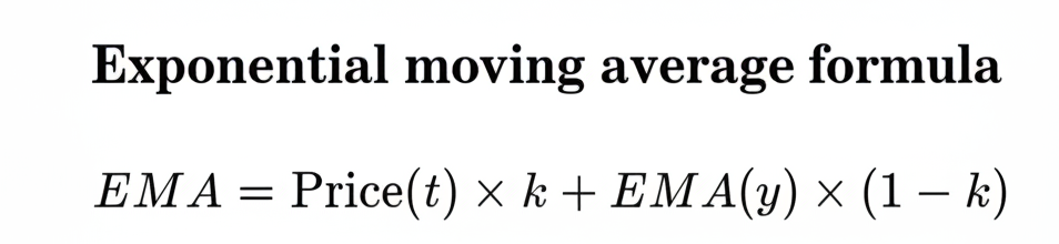
Where:

EMA = Exponential Moving Average for this day (current time) t = current time period k = smoothing factor EMA(y) = Exponential Moving Average for previous day (1-current time)

A common rule of thumb sets k = 2/(n+1) for a window of n, so for 3 days, n = 3, k = 2/4 = 0.5.

We compute the EMA sequentially over the same three days—150, then 70, then 65—and use the last computed EMA as the forecast for the next period.

EMA at the first of the three days (for 150): EMA₁ = 150

EMA at the second day (70): EMA₂ = α×70 + (1−α)×EMA₁ = 0.5×70 + 0.5×150 = 35 + 75 = 110

EMA at the third day (65): EMA₃ = 0.5×65 + 0.5×110 = 32.5 + 55 = 87.5

Then, we use EMA₃ = 87.5 as the forecasted value for the next day.

Note how EMA lands between the two previous methods: SMA = 95, WMA ≈ 80.83, EMA = 87.5.

EMA adapts faster than SMA after a spike because it down-weights older points more aggressively, yet it stays a bit more conservative than a WMA with heavy emphasis on the very last day.

Like this, EMA often performs better in stock prices and other time series with short-term fluctuations. Still, EMA can chase noise if α is set too high, and like the previous two methods, it won’t model seasonality or structural shifts on its own.

To model seasonality or structural shifts, we use more advanced techniques like ARIMA and Holt shines, or even better, regression with traditional machine learning models.

To master forecasting with machine learning, check out our course Forecasting with Machine Learning.

Now that you understand the different moving average forecasting methods, you can choose the right moving average depending on whether you prioritize trend sensitivity or noise reduction.

Advanced tip: Moving averages can be used to create features to forecast using regression models like xgboost, as we will see later in this article. That leverages the power of MA and machine learning, providing in general, more powerful forecasts. Master the creation of features using MA and other techniques with our course Feature Engineering For Time Series Forecasting.

Let’s now implement the different MA methods using Python.

Moving Average Forecasting with Python

Python offers multiple libraries to apply moving average methods. In this article, we’ll cover statsmodels, skforecast and sktime.

Moving Average Forecasting with statsmodels

The statsmodels library is a go-to for traditional statistical forecasting techniques like exponential smoothing, and the moving average models. It provides both simple smoothing tools and full-fledged time series analysis.

Here’s how to implement an Exponential Moving Average forecast in Python using pandas and statsmodels. We’ll use a small synthetic dataset of monthly sales data to demonstrate SMA. We will compare a 3-month simple moving average with Simple Exponential Smoothing on monthly sales data and will plot actuals, smoothed values, and forecasts values.

import pandas as pd
import matplotlib.pyplot as plt
from statsmodels.tsa.api import SimpleExpSmoothing
from pandas.tseries.offsets import MonthEnd

# Example dataset: monthly sales data
data = [200, 220, 250, 270, 300, 280, 310, 330, 350, 370, 390, 410]
df = pd.DataFrame(data, columns=["sales"])
df["month"] = pd.date_range(start="2022-01", periods=len(data), freq="ME")
df.set_index("month", inplace=True)

# --- 3-month Simple Moving Average (for comparison) ---
df["SMA_3"] = df["sales"].rolling(window=3).mean()

# --- Simple Exponential Smoothing (statsmodels) ---
ses_model = SimpleExpSmoothing(df["sales"])
ses_fit = ses_model.fit(optimized=True)   # lets statsmodels choose optimal alpha
df["SES_fitted"] = ses_fit.fittedvalues

# Forecast next 3 months
steps = 3
forecast_index = pd.date_range(start=df.index[-1] + MonthEnd(1), periods=steps, freq="ME")
ses_forecast = ses_fit.forecast(steps)
ses_forecast = pd.Series(ses_forecast, index=forecast_index, name="SES_forecast")

# --- Plotting ---
plt.figure(figsize=(10,6))
plt.plot(df.index, df["sales"], label="Actual", marker="o")
plt.plot(df.index, df["SMA_3"], label="3-Month SMA", linestyle="--")
plt.plot(df.index, df["SES_fitted"], label="SES (fitted)", linestyle="-.", marker="s")
plt.plot(ses_forecast.index, ses_forecast.values, label="SES (forecast)", linestyle="--", marker="o")
plt.title("Simple Exponential Smoothing (statsmodels) vs 3-Month SMA")
plt.xlabel("Month")
plt.ylabel("Sales")
plt.legend()
plt.tight_layout()
plt.show()

In the following plot, we compare actual sales (blue), with a 3-month moving average (broken orange line) and Simple Exponential Smoothing (SES, green line). We see SES tracks the trend more responsively than the SMA, and its forecast flattens at the latest fitted level (red dots).

Moving Average Forecasting with skforecast

While statsmodels focuses on statistical models, skforecast bridges the gap between time series forecasting and machine learning regression. Hence, skforecast allows us to use regression models like Random Forests or XGBoost to predict future values, while incorporatingmoving averages as features.

To master the use of skforecast to forecast with regression models, check out our course Forecasting with Machine Learning.

In this demo, we use skforecast to forecast sales using Random Forest and features obtained using a simple moving average as inputs. We’ll generate synthetic sales data with a trend plus random noise. We will fit a ForecasterRecursive using a Random Forest regression model, and, as features, 5 lag values and a moving-average feature as exogenous input.

import numpy as np
import pandas as pd
import matplotlib.pyplot as plt
from sklearn.ensemble import RandomForestRegressor
from skforecast.recursive import ForecasterRecursive

np.random.seed(42)
n = 50
y = pd.Series(200 + 2 * np.arange(n) + np.random.normal(0, 10, n), index=pd.RangeIndex(n))

# moving-average exog (shifted by 1 to avoid leakage)
window_ma = 5
exog = y.shift(1).rolling(window=window_ma, min_periods=1).mean().to_frame(name=f"ma_{window_ma}")
exog = exog.bfill()  # avoid chained assignment / deprecated fillna(method="bfill")

# forecaster using 5 lags + MA exogenous feature
forecaster = ForecasterRecursive(regressor=RandomForestRegressor(n_estimators=100, random_state=42), lags=5)
forecaster.fit(y=y, exog=exog)

# forecast 10 steps using repeated last MA value for exog
steps = 10
last_ma = exog.iloc[-1, 0]
exog_future = pd.DataFrame([last_ma] * steps, columns=[f"ma_{window_ma}"], index=pd.RangeIndex(start=len(y), stop=len(y)+steps))
forecast = forecaster.predict(steps=steps, exog=exog_future)

# ensure series index for plotting
forecast_series = pd.Series(forecast, index=pd.RangeIndex(start=len(y), stop=len(y)+len(forecast)))

plt.figure(figsize=(10, 5))
plt.plot(y.index, y, label="Historical")
plt.plot(forecast_series.index, forecast_series, "--o", label="Forecast values")
plt.legend()
plt.show()

In the output below, we see a plot displaying historical sales data with forecast values for the next 10 periods extending the trend.

Moving Average Forecasting with sktime

The sktime library provides a unified framework for time series analysis. It’s like an umbrella, that uses statsmodels, sklearn and other libraries under-the-hood, to implement forecasting from a unified API.

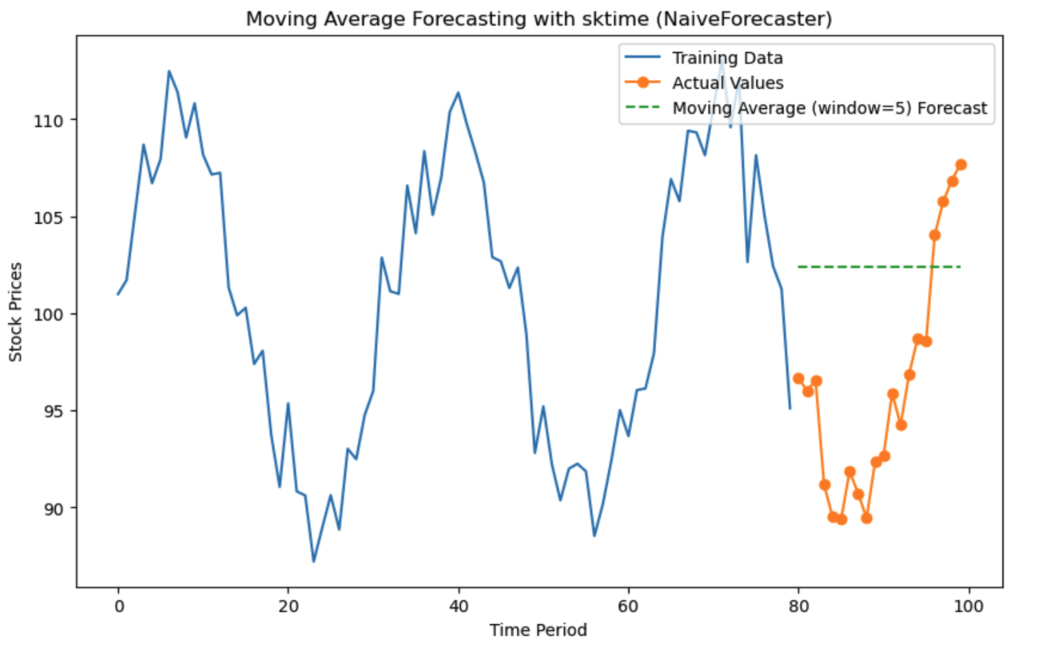
Here’s an example with sktime’s MovingAverageForecaster. We’ll create synthetic stock prices with sinusoidal fluctuations and noise for demonstration. We will us sktime’s NaiveForecaster with a 5-period window to forecast future values for the data.

import pandas as pd
import numpy as np
import matplotlib.pyplot as plt
from sktime.forecasting.naive import NaiveForecaster
from sktime.forecasting.model_selection import temporal_train_test_split

# Generate synthetic stock prices
np.random.seed(42)
time = np.arange(100)
prices = 100 + np.sin(time/5) * 10 + np.random.normal(0, 2, size=len(time))
y = pd.Series(prices)

# Train-test split
y_train, y_test = temporal_train_test_split(y, test_size=20)

# Use NaiveForecaster as a moving-average baseline
window_length = 5
forecaster = NaiveForecaster(strategy="mean", window_length=window_length)
forecaster.fit(y_train)

# Forecast next values
fh = list(range(1, len(y_test) + 1))
y_pred = forecaster.predict(fh)

# Plot
plt.figure(figsize=(10,6))
plt.plot(y_train.index, y_train, label="Training Data")
plt.plot(y_test.index, y_test, label="Actual Values", marker="o")
plt.plot(y_test.index, y_pred, label=f"Moving Average (window={window_length}) Forecast", linestyle="--")
plt.title("Moving Average Forecasting with sktime (NaiveForecaster)")
plt.xlabel("Time Period")
plt.ylabel("Stock Prices")
plt.legend()
plt.show()

In the following output, we see the training data trend along with the actual stock prices for the test period. The moving average forecast appears as a flat line, showing the constant mean of the last 5 observed values.

Evaluating Forecast Performance

Implementing a forecasting method like the moving average model is only half the job. The real test lies in evaluating how well the forecast values match the actual values. Without proper evaluation, we won’t know if our model captures the underlying trends or just produces misleading averages.

When it comes to time series analysis, three widely used error metrics dominate the field:

Mean Absolute Error (MAE)

The MAE calculates the average of absolute differences between forecast and actual values.

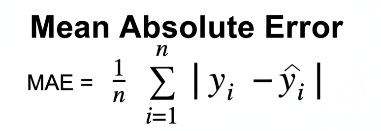
Where:

yi = actual values yi^​ = forecast values n = number of data points

MAE is simple to interpret. If MAE = 5 in a sales forecasting scenario, it means the forecasting technique is off by about 5 units on average.

Root Mean Squared Error (RMSE)

RMSE penalizes large errors more strongly than MAE because it squares the errors before averaging. This makes RMSE especially useful when large deviations are very costly (e.g., forecasting stock prices or medical dosing).

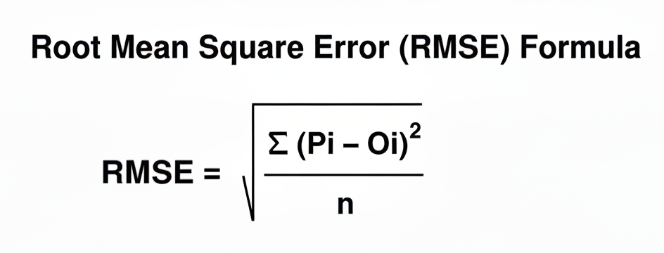
Where:

Pi = Forecast/Predicted Value for the “ith” day Oi = Actual/Original Value for the “ith” day n = total time period

However, RMSE is more sensitive to outliers. As it squares the error terms, a single big outlier can inflate the value much more than MAE would. Therefore, it is widely used in practice when minimizing large errors is critical, but it’s often reported alongside MAE to provide a balanced view of model accuracy.

Mean Absolute Percentage Error (MAPE)

MAPE expresses forecast error as a percentage of the actual values:

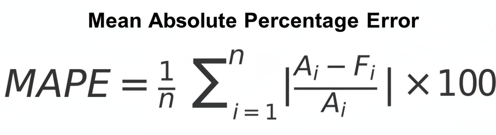
This makes MAPE ideal for business use cases like sales data or demand forecasting, where stakeholders want errors expressed in percentage terms.

We discuss forecast evaluation metrics in much more detail in our course Forecasting with Machine Learning. Check it out to master forecast evaluation.

These metrics can be easily calculated using Python libraries.

Evaluating Forecasts with Python

In this demo, we create synthetic sales data with a slight upward trend and seasonality for model evaluation. We’ll perform a train-test split on our data, and after that, predict future sales using random forests and a combination of lag features and features created from moving average as input. We’ll use a recursive model from skforecast. After training the model, we’ll MAE, RMSE, and MAPE.

import matplotlib.pyplot as plt
from sklearn.ensemble import RandomForestRegressor
from sklearn.metrics import root_mean_squared_error, mean_absolute_error
# NEW import for skforecast 0.17+
from skforecast.recursive import ForecasterRecursive

np.random.seed(42)
time = np.arange(50)
sales = 200 + 2*time + np.random.normal(0, 10, size=len(time))
df = pd.DataFrame({"sales": sales})

# moving-average exog (shifted by 1 to avoid leakage)
window_ma = 5
exog = y.shift(1).rolling(window=window_ma, min_periods=1).mean().to_frame(name=f"ma_{window_ma}")
exog = exog.bfill() # avoid chained assignment / deprecated fillna(method="bfill")

# --- create train/test split so we have true values to evaluate ---
test_size = 10
train_df = df.iloc[:-test_size].copy()
test_df = df.iloc[-test_size:].copy()

train_exog = exog.iloc[:-test_size].copy()
test_exog = exog.iloc[-test_size:].copy()

# --- ForecasterRecursive with RandomForest ---
forecaster = ForecasterRecursive(
regressor=RandomForestRegressor(n_estimators=100, random_state=42),
lags=5
)

# Fit on the train series (skforecast expects a pandas Series)
forecaster.fit(y=train_df["sales"], exog=train_exog)

# Forecast the same horizon as the test set
pred = forecaster.predict(steps=len(test_df), exog=test_exog)

# Ensure pred is a pandas Series with same index as test_df for easy comparison
pred_series = pred.copy()
pred_series.index = test_df.index

# --- Metrics ---
y_true = test_df["sales"].values
y_pred = pred_series.values
rmse = root_mean_squared_error(y_true, y_pred)
mae = mean_absolute_error(y_true, y_pred)

# Safe MAPE calculation (avoid division by zero)
eps = np.finfo(float).eps
mape = np.mean(np.abs((y_true - y_pred) / np.where(y_true == 0, eps, y_true))) * 100
print(f"RMSE: {rmse:.4f}")
print(f"MAE: {mae:.4f}")
print(f"MAPE: {mape:.2f}")

# --- Plot historical, test (true) and forecast ---
plt.figure(figsize=(10, 6))
plt.plot(df.index, df["sales"], label="Historical (all)", alpha=0.4)
plt.plot(train_df.index, train_df["sales"], label="Train", linewidth=2)
plt.plot(test_df.index, test_df["sales"], label="Test (true)", linewidth=2, marker="o")
plt.plot(pred_series.index, pred_series.values,
label="Forecast", linestyle="--", marker="x", linewidth=2)
plt.title("Recursive Forecasting with skforecast and Random Forests")
plt.xlabel("Time Period")
plt.ylabel("Sales")
plt.legend()
plt.show()

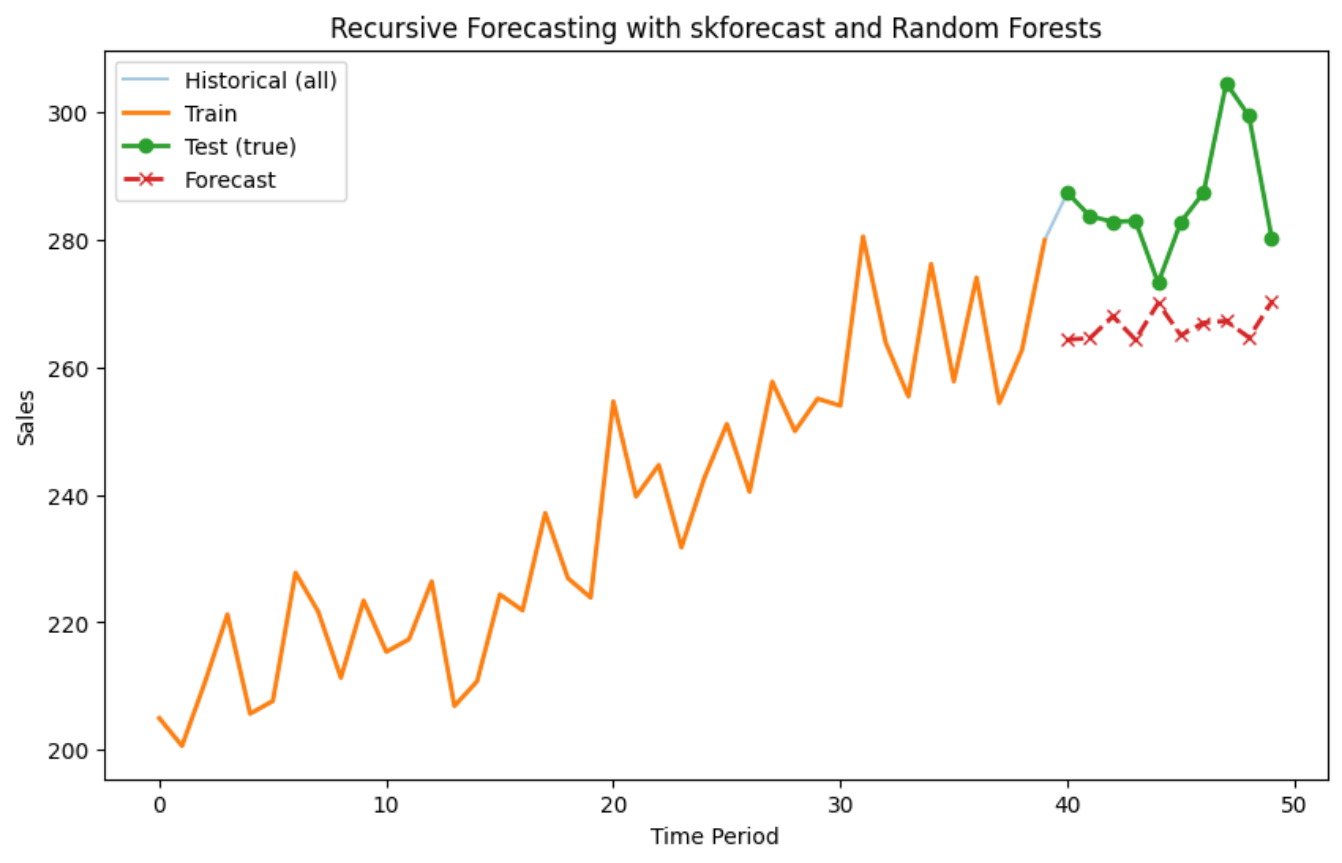
In the following output we see the evaluation metrics (MAE, RMSE, MAPE) that quantify how closely the forecast matches the actual test data.

RMSE: 22.1602
MAE:  19.9190
MAPE: 6.86

The graph shows the training data, actual test values, and the model’s forecast, making it easy to visually compare prediction accuracy.

Conclusion

Moving averages are a simple yet powerful way to analyze time series data. By smoothing short-term fluctuations, it highlights underlying trends and helps forecast future values using past observations.

We can use moving averages the forecast values themselves, or as input features to regression models for forecasting (more in our course Feature Engineering for Time Series Forecasting).

In Python, libraries like statsmodels, skforecast, and sktime make it easy to implement moving average methods, and also compare their performance against advanced models like ARIMA or Holt’s exponential smoothing, using metrics like MAE, RMSE, and MAPE.

While moving averages are not the most advanced forecasting technique, they remain an essential baseline—fast, interpretable, and reliable in many time series forecasting applications.